Frequently Asked Questions - Techniques

ENVI can calculate the Tasseled Cap Transformation of Landsat MSS, TM, and ETM sensor data.  The transforms for each sensor produce a different number of bands.  The MSS transform produces a four-band output file with bands identified as: Soil Brightness Index, Green Veg Index, Yellow Stuff Index, and Non-such Index.  The TM transform produces a three-band output file with bands identified as: Brightness, Greenness, and Third.  The ETM transform produces a six-band output file with bands identified as: Brightness, Greenness, Wetness, Fourth, Fifth, and Sixth.  The user is encouraged to consult the literature for assistance interpreting these data.

ENVI, as of version 5.4.1, does not have a function to apply the Tasseled Cap transform for the Landsat OLI (8) sensor.  In 2014 Muhammad Hasan Ali Baig and colleagues derived transform coefficients for the Landsat OLI sensor.  These coefficients are applied to Landsat OLI bands 2 through 7 (Blue, Green, Red, NIR, SWIR1, and SWIR2) to create new bands identified as: Brightness, Greenness, Wetness, TCT4, TCT5, and TCT6.  Below are the published coefficients to produce the Tasseled Cap transformation for the Landsat OLI sensor.

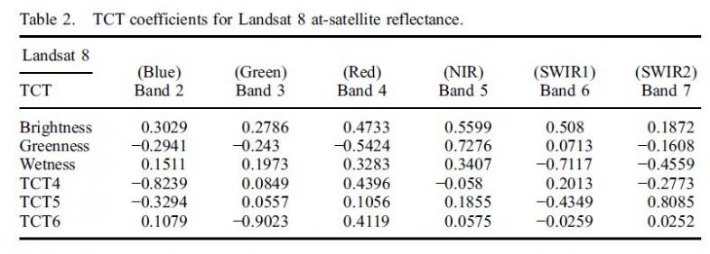
One can use Band Math in ENVI to create new files for the Brightness, Greenness, and Wetness data.  If desired, these three new files can be combined into a single file using the Layer Stacking function in ENVI.  You can see a member of the Yale Center for Earth Observation for a copy of the ENVI Band Math expressions to produce these new layers of data.  They are repeated below for your convenience.

Brightness:     b1*0.3029+b2*0.2786+b3*0.4733+b4*0.5599+b5*0.508+b6*0.1872
Greenness:     b1*(-0.2941)+b2*(-0.243)+b3*(-0.5424)+b4*0.7276+b5*0.0713+b6*(-0.1608)
Wetness:        b1*0.1511+b2*0.1973+b3*0.3283+b4*0.3407+b5*(-0.7117)+b6*(-0.4559)

Note:  The new Coastal Blue band 1 of the OLI sensor is not used in these transforms. 
Note:  Negative values must be enclosed in parenthesis.

Reference:
Muhammad Hasan Ali Baig, Lifu Zhang, Tong Shuai & Qingxi Tong (2014) Derivation of a tasselled cap transformation based on Landsat 8 at-satellite reflectance, Remote Sensing Letters, 5:5, 423-431, DOI: 10.1080/2150704X.2014.915434

To link to the article: http://dx.doi.org/10.1080/2150704X.2014.915434

Often we need to apply the same set of functions to multiple files.  For example, you may want to import a collection of Landsat images, apply radiometric calibration to Top of Atmosphere reflectance, and subset the images to your study area.  Or perhaps you want to import and stack MODIS day-time Land Surface Temperature  (23 per year) for five years.  Then repeat this process for the night-time temperatures.  These can be done individually in ENVI but may take a lot of time and effort .

The ENVI Application Programming Interface (API) can be used to automate many of these repetitive tasks, performing many steps on a large number of files in a batch mode.  These programs (scripts) are based on the IDL programming language and are run in the IDL environment, either by loading the ENVI+IDL program or simply loading IDL by itself.  You can manipulate the ENVI GUI via scripts, or run the scripts without even loading ENVI.  Please see a member of the YCEO staff to learn more.

The ENVI API uses an object-oriented design to operate on data and manipulate the environment.  Use the ENVIRaster object to open a file, or the View function to add a new View in the GUI.  There are a large number of ENVI Tasks that can be called to perform many operations such as stacking layers, classifying an image, or reprojecting a raster.  The API also uses many IDL routines to control looping and other methods of flow control, file searching, directory navigation, etc.

Learn more about programming in the ENVI Help section under Contents | Programming | Programming Guide.  This provides a good introduction and a number of examples to help you get started.  Harris Geospatial Solutions, ENVI’s parent company, has much more detailed information on their site.  Learn about the ENVI Task objects at: https://www.nv5geospatialsoftware.com/docs/ENVITask.html

Detailed function specifications can be found at:   https://www.nv5geospatialsoftware.com/docs/routines-2.html

For those wishing to dig even deeper, check out the IDL Programming guide at:  https://www.nv5geospatialsoftware.com/docs/idl_programming.html

There are times when you may want to capture high resolution screenshots form Google Earth to use in ENVI software.  This could be for background display, ground truthing, or viewing historical imagery.  Basically in Google Earth you will navigate to the area you wish to capture and place markers in each corner.  After saving the image you will use these corner markers to georeferenced your image in ENVI or ArcMap. 

This document is based on information in the UCLA Introduction to GIS page “How To: Add a Google Earth Satellite Image Into ArcMap” located at:
 http://gis.yohman.com/up206a/how-tos/how-to-add-a-google-earth-satellite-image-into-arcmap/

Preparing and capturing the Google image

Follow the Google Earth section on the above link for detailed instructions on placing corner markers.  We recommend using Google Earth Pro, rather than Google Earth, to capture a higher resolution image.  Google Earth Pro is installed on all of the PCs in the YCEO Lab.  You may need to enter your email address as the username and the password GEPFREE.  When you select File | Save | Save Image three buttons are placed above the image.  Click on Map Options to turn off the various map elements.  Click on the Resolution button and select Maximum.  Finally click on the Save Image button to capture the image.

The UCLA page provides instructions on how to georeference the image using ArcMap.  Below are instructions on how to georeference the captured image using ENVI.

Using ENVI

• Open saved image in a new View in ENVI
• From the Toolbox select Geometric Correction | Registration | Registration Image to Map
• Select the RGB bands of image to register
• Increase the resolution to retain more detail:    0.00003513 for example
• Select the Upper Left center point and enter the saved Lon and Lat values
• Click Add Point to save this
• Repeat this step for the three remaining corners
• From GCP Selection dialog
  • Options | Warp (Displayed bands or File)
  • Use Bi Linear interpolation
• Open a new view and display your image

This image could be saved as a GeoPDF and used on a tablet or phone with the Avenza PDF Maps application.

Once you have created a landcover classification in ENVI you may wish to view or work with these data in ArcGIS.  If you include a file extension of “.DAT” as part of the filename you can open this file directly in ArcGIS.  For example, you can open the file MyClass.dat in ArcGIS and you will see the classified image with the colors that you have specified. 

You need to be aware that this is an 8-bit raster image and does not have the attributes of a vector image in ArcGIS, i.e. you cannot use this for zonal statistics, selection by attribute (class), or clipping and buffering other data.  To perform any of these GIS functions you will need to convert the ENVI raster file to an ArcGIS shapefile.

When you use the ENVI Classification Workflow the last step has an option to Export Classification Vectors directly to a shapefile.  While this is easy to do; generally we need to perform many classifications, modifying the training regions along the way.  Also you may want to perform post classification steps such as combining classes.  For these reasons, it is generally better to NOT export the classes at this stage of your analysis.

Once you have performed your image classification(s) and assessed the accuracy of your work,  there is a simple two-step process that you can use to convert the final classified raster data into a vector file structure that can be used in ArcGIS.  Be advised that this could be a time consuming process on large images with many class polygons.

Export to Vector:

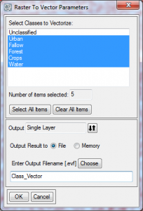From the ENVI Toolbox select Classification | Post Classification | Classification to Vector.  Select your classified image and click OK to open the Raster To Vector Parameters dialog.  You have several options within this dialog; you can select all classes or some subset of them, you can save all of the data to a single layer file or save each class as a separate layer. 

Typically you will select all classes into a single layer file.  Make sure you do not select the default class “Unclassified” or a class labeled “Masked pixels” (created if you applied a mask to your image).  Direct the Output to a Single Layer, enter a new filename such as Class_Vector, and click OK.  This creates an ENVI vector file with the file extension “. EVF”   When opened in the Layer Manager or Data Manager this will display the name RTV(your original classified file name).

Export to Shapefile:

Using the Toolbox select: Vector | Classic EVF to Shapefile.  Select the EVF file from the previous step, enter an appropriate filename for the new shapefile, and click OK.  ENVI will append the ‘.SHP” file extension to your filename.  It may take some time to complete the export, be patient.

Once this is complete, add this shapefile to a map in ArcGIS.  Open the Layer Properties and under the Symbology tab select Categories | Unique Values then click on the button Add All Values to display the separate classes.  ArcGIS will use the ENVI class names but will use its own color scheme.  You can easily change the individual colors and labels here or in the Table of Contents pane.

One important contribution to the understanding of a landscape is the incoming solar radiation, or insolation, that is available at the surface.  While one could use the global average of 1366 watts/m², actual values are generally much lower.  On a global scale the controlling variables are the latitude, distance from the sun, and time of year.  At the local level elevation, slope and aspect are major factors in determining the amount of energy available.   You will need ArcGIS version 9.2 or greater with the Spatial Analysis extension.

The Solar Analyst module in ArcGIS can be used to calculate Watt-Hours/meter² at the surface at the local scale.  Inputs to this process are a digital elevation model (DEM), the latitude of the scene center, and the date and time that you wish to accumulate insolation.  You can specify a portion of a day, or a range of days such as a week or month.

For purposes of this document, we will use the Solar Analyst to accumulate the energy striking the surface for the one hour prior to the acquisition of a Landsat image.  You could then compare the amount of energy available at the surface, to the brightness-temperature derived from the Landsat thermal band.  Alternatively you could adjust the parameters to compare the amount of energy available over a growing season, to the local land cover.

Required inputs

The most important requirement is an accurate, georeferenced DEM dataset.  If you do not have one for your study area, use the DEM FAQ on this site to help you locate one.  Make note of the scene center latitude.   The Solar Analyst module may not determine this automatically when the dataset is opened.

For this example, the other required inputs are the Julian date and the local time of day of image acquisition.  As a reminder, the Julian day of year is simply the sequential number from 1 to 365 (or 366 if a leap year).  You can use the Julian Data Calendar, on the YCEO Lab workstation desktops, to calculate this.  Local time of day is a function of latitude.  The Landsat orbit is designed to cross the equator at approximately noon local time.  An orbit takes approximately 90 minutes, or 45 minutes from pole to pole.  A rough estimate of the local time is fine.

Create new data layers

Begin this process by loading ArcGIS and activating the Spatial Analysis extension if necessary.  Add your DEM to the new empty map.  Open ArcToolbox and select Spatial Analyst Tools | Solar Radiation | Area Solar Radiation.

You will input or adjust the following values:

• Select the DEM for the Input Raster. 
• Enter the name WattsTot for the Output global radiation raster. 
• Latitude should be prefilled from the DEM; if not, enter the latitude of the scene center
• Set the Sky size/Resolution to 1600
• For Time configuration select “Within a day”
• Day number of the year is the Julian date of the image
• End time is the time of image acquisition derived earlier in Local Solar Time
• Start time is one hour prior to image acquisition using Local Solar Time.

Note:  This will create a new ArcGRID data layer for the total watts/m² for the surface.  If you are interested in its two components, direct and diffuse energy, do the following.  Scroll down to the Optional outputs section and click on the down arrow to open this section.  You can create data layers for direct radiation and diffuse radiation using filenames WattsDir and WattsDiff respectively.

There are several radiation parameters that use the default values for a generally clear sky.  These could be modified as part of a future research project, or if the scene conditions warrant a change.  Variables include Transmittivity (0.5) and Diffuse proportion (0.3).  The Uniform Sky model could be changed to the Standard Overcast Sky model.  Also the Zenith and Azimuth divisions have been set to 8.  See the help section of the Area Solar Radiation window in ArcGIS for more information.

After reviewing all of the parameters click OK.  This process may take several hours to complete. When this is finished you will have up to three new ArcGRID layers in your map.  You may want to convert these data to the TIFF format for use in other geospatial software.