Frequently Asked Questions - Landsat

This is a very brief description of the Landsat sensors.  Users are encouraged to review sensor information before working with these data.  A few suggested sites are the USGS Landsat Program site and the NASA Landsat Users Handbook.

Basic Image Characteristics

There are four generations of sensors used in the Landsat program.  The Multi Spectral Scanner (MSS) mission ran from 1972 to 1993 and had four spectral channel covering the green, red, and (2) near infrared channels.  The spatial resolution was 57 or 60 meters.

The Landsat Thematic Mapper (TM) mission began in the mid-80’s and Landsat 5 finally ended November 2012.  This sensor features seven spectral channels at 30 meters spatial resolution.

The Landsat 7 Enhanced Thematic Mapper (ETM) mission began in 1999 and is still operational.  It features the same spectral channels as the TM sensor, with the addition of a second thermal channel and a 15 meter panchromatic channel.  On May 31, 2003 the ETM scan line corrector failed and ETM images since that time are missing large portions each scene.  On USGS sites these images are designated as SLC-Off and use of these images is generally not recommended.

The Landsat 8 mission began in the spring of 2013.  This features 11 bands of data, many similar to the ETM mission.  The primary file in the Optical Land Imager (OLI) sensor has 7 bands of data at 30m resolution; Coastal Blue, Blue, Green, Red, NIR, SWIR1 and SWIR2.  It also has a 30m Cirrrus file and a 15m Panchromatic file.  The Thermal InfraRed (TIR) sensor has 2 bands of data with 100m resolution.  Users are advised to only use the first (band 10) TIR band in their research.

Landsat 8 Pre-WRS-2

The Landsat 8 program began acquiring images in March of 2013 once the final sensor calibration checkout was completed .  This was before the satellite actually arrived at its final orbital position on April 11, 2013.  As a result, these scenes do not properly align to the designated Path/Row footprint and each cell covers a slightly smaller area.  These scenes are identified as Pre-WRS-2 and we do not recommend using these for studies over time.

Worldwide Reference System

The Worldwide Reference System (WRS) is used to identify the path and row of each Landsat image.  The path is the descending orbit of the satellite.  Each path is segmented into 119 rows, from north to south.  The Landsat MSS sensor had a swath width of 180 km and global coverage required 251 paths.  The Landsat TM, ETM and OLI sensors have a swath width of 185 km and require only 233 paths for complete coverage.  MSS and TM scenes share common rows, but in most cases the paths will be different.  Because of this difference, MSS scenes are identified using WRS I while TM, ETM and OLI scenes use WRS II path/row designations.  The data archive section of the CEO web site uses the WRS II designation for all path/row images.

The USGS has begun to reprocess all of the Landsat images in their archive.  These images will be released as Collection 1 data and be designated as either Tier 1 or Tier 2.  All Collection 1 data will share common radiometric and geometric parameters.  In the future, if these need to be adjusted, then all archived images will be reprocessed and a new Collection will be released.

Tier 1 data have the highest radiometric and positional quality.  They have precision terrain processing and have been inter-calibrated across the Landsat sensors.  The USGS recommends using Tier 1 data for all future time-series analysis.

Tier 2 data are still very good images.  They may have more cloud cover, affecting the radiometric calibration and obscuring ground control points within the scenes.

The USGS will also release new higher level Landsat data such as Surface Reflectance and several spectral indices.  You can learn more about these products at:  http://landsat.usgs.gov//landsat_cdr_ecv.php

Collection 1 data will become available starting in August 2016.   The USGS will begin with the Landsat 4-5 TM and 7 ETM+ scenes, working backward through time.  They plan to begin processing Landsat 8 data in November.  You can learn more about this new process at the USGS Landsat Collection page.

Initially these Collection 1 data will only be available on the USGS Earth Explorer site at: http://earthexplorer.usgs.gov/.  Click on the Data Sets tab then expand the Landsat Archive section to view the Collection data.  You will also be able to slect the Pre-Collection data that we have been using for years.  In the future the USGS will also make Collection data available through the GloVis site

There are many sites that you can use to locate and obtain Landsat satellite imagery.  Two recommended sites are EarthExplorer and GLOVIS by the USGS.   You will find a broad collection of Landsat data spanning the entire time of the program, beginning in the early 1970’s.  The user interface and download processes are a bit different for each site.  More information about each is listed below.

There are several international sources of Landsat images which typically charge $1,000 or more per scene.  You may also find various government or non-profit organizations that maintain an archive of images for their region which can be shared with the public, or at least with research collaborators.  Locating and accessing these sites is beyond the scope of this document.

Earth Explorer

The Earth Explorer site at: http://earthexplorer.usgs.gov/ includes many types of data in addition to Landsat images.  Begin on the Search Criteria tab to define the location you are interested in.  There are many ways to do this; click on the map to create a polygon, upload a shapefile, select a Landsat Path/Row, etc.  While still on this tab define a time range and adjust the Result Options to determine how many images may be presented to you. 

Next click on the Data Sets tab and expand the Landsat Archive section.  You can select the Landsat sensor(s) you are interested in, or the Collection data and higher products as they become available  You may need to modify the dates and/or the number of results to find appropriate data.  (Note that there are many other types of data available on this site.)

Click on the Results tab to view images that meet your criteria.  From this page you can look at browse images, inspect the meta data, display the footprint to see the scene coverage, download an image, or place an order.  You must register on the site to access the images.

GLOVIS

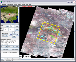The USGS Global Visualization Viewer GLOVIS site at: http://glovis.usgs.gov/ has Landsat data, as well as ASTER and some MODIS satellite images.  Select the appropriate image collection e.g. Landsat Archive | Landsat 4 – 5 TM and then navigate to the region you are interested in.  You can use the Prev Scene and Next Scene buttons to scroll through the available images by date. 

When you have located an image you wish to work with, click the Add button in the lower left to make it available for ordering.  Users can select several images and place them in a “cart” for ordering.  Most data are available for immediate download once they are “Added” to your cart.  For these images, make sure you select the Level 1 Product.  In other cases, the image request is submitted to the USGS and when the data are available the user will get an email with a link to retrieve the data.  This may take a few hours to a few days.  

Note:  When you enter the site your browser must allow pop-up windows so that the Visualization Viewer window can open.  Each user must register on this site before downloading or ordering images.

Landsat data provided by the USGS are distributed as a single file in an archived and zipped “.TAR.GZ” format.   These files must be extracted and uncompressed before you can use them.

After downloading a file move it to a separate folder in your user section of the server.  Double click on it to load the program 7-Zip, showing the “.tar” file.  Right-click on the “.tar” file and select Open Inside to display the detail data files.  Click on the blue Extract icon and select the destination folder to extract the individual files that comprise the entire image.  Each data layer is a separate TIF image file.  There are also two text files with the same base filename but ending with _GCP.TXT and _MTL.TXT.  This file structure is referred to as “GeoTIFF with Meta data”.

Level 1 Image

ENVI can directly and easily open data in this USGS format.  Each data layer will end in …_T1_B1.TIF (or B2.TIF, B3.TIF, etc.).   From the ENVI main menu select File | Open and navigate to the _MTL.TXT file.  ENVI will automatically open the Landsat image with all bands in the correct order.  The reflective bands are placed in one file, the thermal band(s) in another file.  There will be a 15m panchromatic file for ETM and OLI sensors and a 30m Cirrus file for the OLI sensor.

While you can work with these data as they are, ENVI has only created a temporary virtual layer stack that is constantly resampled as you move around the image.  You should save each file as a new dataset.  From the ENVI main menu select File | Save As, pick the file you wish to save, and in the Save File As Parameters dialog select the Output Format ENVI.  Then in the Output Filename box navigate to your work area and enter an appropriate file name.  Once this is saved as a new file, the uncompressed “.TIF” files and the “.tar” file can be deleted.

Level 2 Surface Reflectance Product

The Level 2 Surface Reflectance product has been converted by the USGS from digital numbers to surface reflectance.  Each data layer will end in …_T1_sr_band1.TIF (or band2.TIF, band3.TIF, etc.).  As of this writing the USGS  provides the original Level 1 metadata TXT file, which does not correspond to the supplied Level 2 data files.  As a result, ENVI cannot open these data files directly from the MTL.TXT file as it can with Level 1 data described above.  You must open each data layer individually, then create a layer stack, and finally save the result as a new file.

Open all 6 or 7 … _T1_sr_bandn.TIF files in ENVI as grayscale datasets.  In the Toolbox search box type layer to find the Layer Stack tool and open it.  Click on the Import button and add the 6 or 7 images.  Carefully check that the images are in the correct order, i.e. band 1 is followed by band 2, band 3, etc.  If they are not in the correct order click on the Reorder button and rearrange them.  Click OK and save this as a new ENVI file with a meaningful name such as the date in yyyymmdd.dat format.

The Landsat Thematic Mapper (TM) and Enhanced Thematic Mapper Plus (ETM+) sensors capture reflected solar energy, convert these data to radiance, then rescale this data into an 8-bit digital number (DN) with a range between 0 and 255.  It is possible to manually convert these DNs to ToA Reflectance using a two-step process.  The first step is to convert the DNs to radiance values using the bias and gain values specific to the individual scene you are working with.  The second step converts the radiance data to ToA reflectance.  

The Landsat 8 OLI sensor is more sensitive so these data are rescaled into 16-bit DNs with a range from 0 and 65536.  Also these data have been converted to reflectance, rather than radiance, so DNs can be manually converted to Reflectance in a single step.

ENVI can easily convert Landsat data from the USGS in the “USGS GeoTIFF with Metadata” format in a single step.  This process is described in Section 1 of this document.  For other Landsat data, or other remote sensing software, you may need to apply the manual conversion processes described in Section 2 or 3 below.

1. ENVI and USGS GeoTIFF with Metadata format data

The USGS now provides data in the GeoTIFF with Metadata format.  ENVI software can easily convert the optical band data to ToA reflectance values when you open the USGS file that ends with “_MTL.TXT”.  ENVI will automatically open the Landsat image as multiple files with the 6 or 7 bands of optical data as one of several files.

To create a reflectance data file using ENVI Classic, from the ENVI main menu bar select Basic Tools |Preprocessing |Calibration Utilities |Landsat Calibration.  Select the optical data file (it has six or seven bands) and the ENVI Landsat Calibration dialog should open with all of the calibration parameters filled in.  Click on the Reflectance radio button and enter an output file name.

For ENVI Standard, select from the Toolbox | Radiometric Correction | Radiometric Calibration.  Select the optical data file and the Radiometric Calibration dialog opens.  Under Calibration Type choose Reflectance and save the new file.  As a reminder, reflectance values range from 0.0 to 1.0 and are stored in floating point data format.

2. Manually Converting Landsat 8 OLI data to ToA Reflectance:

These data can be converted to ToA Reflectance using rescaling factors and parameters found in the metadata file (MTL.txt) provided with the data.  The formulas and detailed explanations can be found on the USGS site: Using the USGS Landsat 8 Product.  You should use the formula that includes a correction for the sun angle.

3. Manually Converting Landsat TM and ETM data to ToA Reflectance:

This is a two-step process.  First you must convert DNs to radiance values, then you need to convert these radiance values to reflectance values.  For each scene you need to know the distance between the sun and earth in astronomical units, the day of the year (Julian date), and solar zenith angle.  This information can also be found in Chapter 11 of the Landsat 7 Users Handbook .  Sections of the Landsat 7 Users Handbook have been included in this document to guide you.

3.1. DN to Radiance

There are two formulas that can be used to convert DNs to radiance; the method you use depends on the scene calibration data available in the header file(s).  One method uses the Gain and Bias (or Offset) values from the header file.  The longer method uses the LMin and LMax spectral radiance scaling factors.   Look for a file name such as LT5171034009024510.WO, or a file with .met or .txt as the file extension.  For ETM+ images this information may be in a file name such as L71171035_03520000905_htm.fst.

Appropriate calibration parameter files are available on the Landsat Calibration page at the USGS.

3.1.1.Gain and Bias Method

The formula to convert DN to radiance using gain and bias values is:

Where:

L_λ  is the cell value as radiance
DN  is the cell value digital number
gain is the gain value for a specific band
bias is the bias value for a specific band

The ENVI formula in Band Math will look like:

0.05518 * (B1) + 1.2378   

using a scene specific gain value of 0.05518 and an offset value of 1.2378.  In the Band Pairing dialog you should match B1 with the appropriate optical band.

3.1.2.Spectral Radiance Scaling Method

The formula used in this process is as follows:

Where:

L_λ  is the cell value as radiance
QCAL = digital number
LMIN_λ = spectral radiance scales to QCALMIN
LMAX_λ = spectral radiance scales to QCALMAX
QCALMIN = the minimum quantized calibrated pixel value
     (typically = 1)
QCALMAX = the maximum quantized calibrated pixel value
     (typically = 255)

3.2. Radiance to ToA Reflectance

From the Landsat 7 Users Handbook – Chapter 11:

Where:
                ρ_λ = Unitless plantary reflectance
                L_λ= spectral radiance (from earlier step)
                d = Earth-Sun distance in astronmoical units
                ESUN_λ = mean solar exoatmospheric irradiances
                θ_s = solar zenith angle

The solar zenith angle can be calculated using the University of Oregon Solar Poistion Calulator.

The following tables are from the Landsat & Users Handbook – Chapter 11

http://landsathandbook.gsfc.nasa.gov/data_prod/prog_sect11_3.html

.

The Landsat Thematic Mapper (TM) and Enhanced Thematic Mapper Plus (ETM+) sensors acquire Thermal InfraRed (TIR) data and store this information as a digital number (DN) with a range between 0 and 255.  The Landsat 8 OLI sensor stores these data as DNS with a range from 0 to 65536.  ENVI Standard can easily convert these DNs to degrees Kelvin.

You need to open the original USGS supplied file in USGS GeoTIFF with Metatdata format. Open the file that ends with “_MTL.TXT”.  ENVI will automatically open the Landsat image as multiple files.  For Landsat TM there will be a single TIR band, for ETM and OLI there will be two bands of TIR data.

Using ENVI Standard, select from the Toolbox | Radiometric Correction | Radiometric Calibration.  Select the TIR data file and the Radiometric Calibration dialog opens.  Under Calibration Type choose Brightness Temperature and save the new file. 

Albedo is an important property of the Earth surface heat budget. A simple definition of albedo (a) is the average reflectance of the sun’s spectrum. This unitless quantity has values ranging from 0 to 1.0 and will vary based on the land cover. For example snow would have a high value and coniferous forests a low value.

The input to the albedo calculation will be a Landsat image that has been converted from digital numbers to Top of Atmosphere (TOA) reflectance. Please refer to the FAQ Converting Digital Numbers to Top of Atmosphere Reflectance on this site for detailed instructions on how to accomplish this.

Liang (2000) developed a series of algorithms for calculating albedo from various satellite sensors. His Landsat formula to calculate Landsat shortwave albedo was normalized by Smith (2010) and is presented below.

    Where ρ represents Landsat bands 1,3,4,5, and 7. Note that Landsat band 2 (green) is not used.

This formula can be implemented in ENVI using Band Math as:

((0.356*B1) + (0.130*B2) + (0.373*B3) + (0.085*B4) + (0.072*B5) -0.018) / 1.016

Note: If you have areas outside of the image scene or mask area with values of 0.0 these will have a negative value. You should apply a mask to convert these fill values to NaN (Not a Number) before or after calculating albedo.

References

Liang, S. 2000. “Narrowband to broadband conversions of land surface albedo I algorithms.” Remote Sensing of Environment 76, 213-238.

Smith, R.B. 2010. “The heat budget of the earth’s surface deduced from space” available on this site

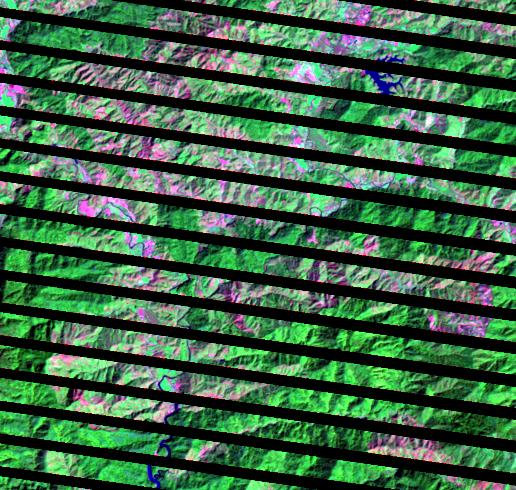
On 31 May 2003 the Landsat 7 Enhanced Thematic Mapper (ETM) sensor had a failure of the Scan Line Corrector (SLC).  Since that time all Landsat ETM images have had wedge-shaped gaps on both sides of each scene, resulting in approximately 22% data loss.  These images are available for free download from the USGS GloVis website and are found in the L7 SLC-off collection. 

Scaramuzza, et al (2004) developed a technique which can be used to fill gaps in one scene with data from another Landsat scene.  A linear transform is applied to the “filling” image to adjust it based on the standard deviation and mean values of each band, of each scene.  More information about this technique can be found in the USGS article "SLC Gap-Filled Products, Phase One Methodology". 

This document assumes you are using ENVI software and have installed the plugin landsat_gapfill.sav in the proper ENVI install folder(s).   At this point the Gapfill plugin is not available in the ENVI Code Library but a copy can be found at:
    https://docs.google.com/file/d/0B3e_wo8OTO47b3c4ZHNyV0NmUkk/edit?usp=sha...

	9 Feb 2011 image		9 Feb image filled with 25 Feb 2011 image

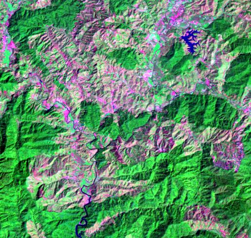This document describes how to apply this gap filling technique using an add-on module in the ENVI software.  Guidelines are provided for the selection of images that may produce a quality gap-filled Landsat ETM image.  Below you can see an example of this gap-filling technique as applied to a pair of Landsat ETM images from Path 130 Row 45 acquired on 9 and 25 February 2011.

Image Selection

Your first step is to find appropriate images that can be used to produce a quality result.  Care must be taken when evaluating images for this technique.  At a minimum, these images must be accurately co-registered.  Images obtained from the USGS GloVis site in the “GeoTIFF plus Metadata” format have all been terrain corrected so this will not be an issue when using these images.  If you obtain images from other sources you will need to co‑register these images before proceeding.

Optimal results will be obtained if both images are free of clouds and shadows, or snow and ice.  Generally you should try to find images that have been acquired as close in time as possible.  Landsat ETM repeats coverage of an area every 16 days.  For some studies you may be able to use images approximately one year apart.  This would eliminate any scene variation due to sun angle and distance.

Pay attention to local landscape changes such as plant phenology and harvesting practices.  For example, you should not combine images acquired before and after leaf-out in areas with deciduous forests.  Also consider major events that may change the landscape, such as tsunamis or hurricanes.  You should not use images from before and after a major change event to produce a meaningful gap-filled image.

Preparation

In some cases you may want to perform pre-processing functions such as atmospheric correction or conversion of digital numbers to top-of-atmosphere reflectance on these images.  Because these are scene-specific operations they cannot be applied correctly to a blended multi-date image.  Any pre-processing functions such as these must be done before using this image gap-fill routine.

Finally, you need to evaluate which image will be the master scene to be filled, and which will be used to fill in the gaps.  This is a subjective decision based on your review of the selected scenes.  Take the time to view the scenes using different band combinations, perhaps even linking the two scenes.

Image Gap Filling

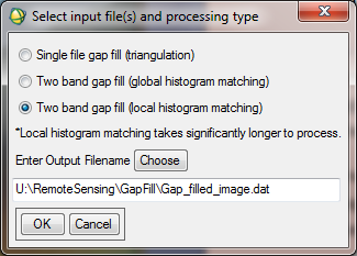Use the ENVI software program to open the two Landsat ETM images you have selected above.  If you are using ENVI Standard interface look under Toolbox | Extensions | landsat_gapfill.  If using ENVI Classic, from the main menu bar, select Basic Tools | Preprocessing | Data-Specific Utilities | Landsat TM | Landsat Gapfill.  This will open the Select input file(s) and processing type dialog.  You should only use the option Two band gap-fill (Local histogram matching), the other options do not perform as well.  Next, click on the Choose button to navigate to a folder and enter an output filename. 

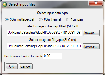Click OK to open the Select input files dialog box.  Make sure you select the appropriate image data type; 30m multispectral, 60m thermal, or 15m pan.  Select your master image as the image to be gap filled then select the second image; you will use this to fill gaps in the first image.  Click OK and wait for this to complete.

Restore Data Type

The gap-filling technique produces an output image with a 4-byte floating point data type.  If you are working with TOA Reflectance values, then your work is complete.  However if you are working with the original digital numbers, you should convert these data back to integers.  This will reduce the file size by 75% and make all subsequent processing faster.

From the ENVI Classic menu bar, select Basic Tools | Band Math or from the ENVI Standard Toolbox select Band Ratio | Band Math and enter the expression:    byte(round(b1))
Click OK and select the button Match Variable to Input File to convert the entire dataset at once.  Save this as a new file and delete the gap-filled image created in Section 3 above.

The USGS provides on-demand processing of Landsat 4, 5, and 7 images to create Climate Data Records (CDR)s and Essential Climate Variables (ECV)s.  The CDRs are Landsat scenes that have been atmospherically corrected and converted to Surface Reflectance.  ECVs are spectral indices derived from the CDRs and include vegetation, moisture and burn ratio indices.

Before ordering these data you should read the USGS CDR Product Guide and/or ECV Product Guide.  Data orders are placed using the USGS ESPA Ordering Interface.  You will need to provide a text file with a list of desired scenes using the USGS naming conventions.  The ESPA User Guide provides information on how to construct and submit an order.