Frequently Asked Questions
Landsat
This is a very brief description of the Landsat sensors. Users are encouraged to review sensor information before working with these data. A few suggested sites are the USGS Landsat Program site and the NASA Landsat Users Handbook.
Basic Image Characteristics
There are four generations of sensors used in the Landsat program. The Multi Spectral Scanner (MSS) mission ran from 1972 to 1993 and had four spectral channel covering the green, red, and (2) near infrared channels. The spatial resolution was 57 or 60 meters.
The Landsat Thematic Mapper (TM) mission began in the mid-80’s and Landsat 5 finally ended November 2012. This sensor features seven spectral channels at 30 meters spatial resolution.
The Landsat 7 Enhanced Thematic Mapper (ETM) mission began in 1999 and is still operational. It features the same spectral channels as the TM sensor, with the addition of a second thermal channel and a 15 meter panchromatic channel. On May 31, 2003 the ETM scan line corrector failed and ETM images since that time are missing large portions each scene. On USGS sites these images are designated as SLC-Off and use of these images is generally not recommended.
The Landsat 8 mission began in the spring of 2013. This features 11 bands of data, many similar to the ETM mission. The primary file in the Optical Land Imager (OLI) sensor has 7 bands of data at 30m resolution; Coastal Blue, Blue, Green, Red, NIR, SWIR1 and SWIR2. It also has a 30m Cirrrus file and a 15m Panchromatic file. The Thermal InfraRed (TIR) sensor has 2 bands of data with 100m resolution. Users are advised to only use the first (band 10) TIR band in their research.
Landsat 8 Pre-WRS-2
The Landsat 8 program began acquiring images in March of 2013 once the final sensor calibration checkout was completed . This was before the satellite actually arrived at its final orbital position on April 11, 2013. As a result, these scenes do not properly align to the designated Path/Row footprint and each cell covers a slightly smaller area. These scenes are identified as Pre-WRS-2 and we do not recommend using these for studies over time.
Worldwide Reference System
The Worldwide Reference System (WRS) is used to identify the path and row of each Landsat image. The path is the descending orbit of the satellite. Each path is segmented into 119 rows, from north to south. The Landsat MSS sensor had a swath width of 180 km and global coverage required 251 paths. The Landsat TM, ETM and OLI sensors have a swath width of 185 km and require only 233 paths for complete coverage. MSS and TM scenes share common rows, but in most cases the paths will be different. Because of this difference, MSS scenes are identified using WRS I while TM, ETM and OLI scenes use WRS II path/row designations. The data archive section of the CEO web site uses the WRS II designation for all path/row images.
The USGS has begun to reprocess all of the Landsat images in their archive. These images will be released as Collection 1 data and be designated as either Tier 1 or Tier 2. All Collection 1 data will share common radiometric and geometric parameters. In the future, if these need to be adjusted, then all archived images will be reprocessed and a new Collection will be released.
Tier 1 data have the highest radiometric and positional quality. They have precision terrain processing and have been inter-calibrated across the Landsat sensors. The USGS recommends using Tier 1 data for all future time-series analysis.
Tier 2 data are still very good images. They may have more cloud cover, affecting the radiometric calibration and obscuring ground control points within the scenes.
The USGS will also release new higher level Landsat data such as Surface Reflectance and several spectral indices. You can learn more about these products at: http://landsat.usgs.gov//landsat_cdr_ecv.php
Collection 1 data will become available starting in August 2016. The USGS will begin with the Landsat 4-5 TM and 7 ETM+ scenes, working backward through time. They plan to begin processing Landsat 8 data in November. You can learn more about this new process at the USGS Landsat Collection page.
Initially these Collection 1 data will only be available on the USGS Earth Explorer site at: http://earthexplorer.usgs.gov/. Click on the Data Sets tab then expand the Landsat Archive section to view the Collection data. You will also be able to slect the Pre-Collection data that we have been using for years. In the future the USGS will also make Collection data available through the GloVis site
There are many sites that you can use to locate and obtain Landsat satellite imagery. Two recommended sites are EarthExplorer and GLOVIS by the USGS. You will find a broad collection of Landsat data spanning the entire time of the program, beginning in the early 1970’s. The user interface and download processes are a bit different for each site. More information about each is listed below.
There are several international sources of Landsat images which typically charge $1,000 or more per scene. You may also find various government or non-profit organizations that maintain an archive of images for their region which can be shared with the public, or at least with research collaborators. Locating and accessing these sites is beyond the scope of this document.
Earth Explorer
The Earth Explorer site at: http://earthexplorer.usgs.gov/ includes many types of data in addition to Landsat images. Begin on the Search Criteria tab to define the location you are interested in. There are many ways to do this; click on the map to create a polygon, upload a shapefile, select a Landsat Path/Row, etc. While still on this tab define a time range and adjust the Result Options to determine how many images may be presented to you.
Next click on the Data Sets tab and expand the Landsat Archive section. You can select the Landsat sensor(s) you are interested in, or the Collection data and higher products as they become available You may need to modify the dates and/or the number of results to find appropriate data. (Note that there are many other types of data available on this site.)
Click on the Results tab to view images that meet your criteria. From this page you can look at browse images, inspect the meta data, display the footprint to see the scene coverage, download an image, or place an order. You must register on the site to access the images.
GLOVIS
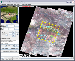 The USGS Global Visualization Viewer GLOVIS site at: http://glovis.usgs.gov/ has Landsat data, as well as ASTER and some MODIS satellite images. Select the appropriate image collection e.g. Landsat Archive | Landsat 4 – 5 TM and then navigate to the region you are interested in. You can use the Prev Scene and Next Scene buttons to scroll through the available images by date.
When you have located an image you wish to work with, click the Add button in the lower left to make it available for ordering. Users can select several images and place them in a “cart” for ordering. Most data are available for immediate download once they are “Added” to your cart. For these images, make sure you select the Level 1 Product. In other cases, the image request is submitted to the USGS and when the data are available the user will get an email with a link to retrieve the data. This may take a few hours to a few days.
Note: When you enter the site your browser must allow pop-up windows so that the Visualization Viewer window can open. Each user must register on this site before downloading or ordering images.
Landsat data provided by the USGS are distributed as a single file in an archived and zipped “.TAR.GZ” format. These files must be extracted and uncompressed before you can use them.
After downloading a file move it to a separate folder in your user section of the server. Double click on it to load the program 7-Zip, showing the “.tar” file. Right-click on the “.tar” file and select Open Inside to display the detail data files. Click on the blue Extract icon and select the destination folder to extract the individual files that comprise the entire image. Each data layer is a separate TIF image file. There are also two text files with the same base filename but ending with _GCP.TXT and _MTL.TXT. This file structure is referred to as “GeoTIFF with Meta data”.
Level 1 Image
ENVI can directly and easily open data in this USGS format. Each data layer will end in …_T1_B1.TIF (or B2.TIF, B3.TIF, etc.). From the ENVI main menu select File | Open and navigate to the _MTL.TXT file. ENVI will automatically open the Landsat image with all bands in the correct order. The reflective bands are placed in one file, the thermal band(s) in another file. There will be a 15m panchromatic file for ETM and OLI sensors and a 30m Cirrus file for the OLI sensor.
While you can work with these data as they are, ENVI has only created a temporary virtual layer stack that is constantly resampled as you move around the image. You should save each file as a new dataset. From the ENVI main menu select File | Save As, pick the file you wish to save, and in the Save File As Parameters dialog select the Output Format ENVI. Then in the Output Filename box navigate to your work area and enter an appropriate file name. Once this is saved as a new file, the uncompressed “.TIF” files and the “.tar” file can be deleted.
Level 2 Surface Reflectance Product
The Level 2 Surface Reflectance product has been converted by the USGS from digital numbers to surface reflectance. Each data layer will end in …_T1_sr_band1.TIF (or band2.TIF, band3.TIF, etc.). As of this writing the USGS provides the original Level 1 metadata TXT file, which does not correspond to the supplied Level 2 data files. As a result, ENVI cannot open these data files directly from the MTL.TXT file as it can with Level 1 data described above. You must open each data layer individually, then create a layer stack, and finally save the result as a new file.
Open all 6 or 7 … _T1_sr_bandn.TIF files in ENVI as grayscale datasets. In the Toolbox search box type layer to find the Layer Stack tool and open it. Click on the Import button and add the 6 or 7 images. Carefully check that the images are in the correct order, i.e. band 1 is followed by band 2, band 3, etc. If they are not in the correct order click on the Reorder button and rearrange them. Click OK and save this as a new ENVI file with a meaningful name such as the date in yyyymmdd.dat format.
The Landsat Thematic Mapper (TM) and Enhanced Thematic Mapper Plus (ETM+) sensors capture reflected solar energy, convert these data to radiance, then rescale this data into an 8-bit digital number (DN) with a range between 0 and 255. It is possible to manually convert these DNs to ToA Reflectance using a two-step process. The first step is to convert the DNs to radiance values using the bias and gain values specific to the individual scene you are working with. The second step converts the radiance data to ToA reflectance.
The Landsat 8 OLI sensor is more sensitive so these data are rescaled into 16-bit DNs with a range from 0 and 65536. Also these data have been converted to reflectance, rather than radiance, so DNs can be manually converted to Reflectance in a single step.
ENVI can easily convert Landsat data from the USGS in the “USGS GeoTIFF with Metadata” format in a single step. This process is described in Section 1 of this document. For other Landsat data, or other remote sensing software, you may need to apply the manual conversion processes described in Section 2 or 3 below.
1. ENVI and USGS GeoTIFF with Metadata format data
The USGS now provides data in the GeoTIFF with Metadata format. ENVI software can easily convert the optical band data to ToA reflectance values when you open the USGS file that ends with “_MTL.TXT”. ENVI will automatically open the Landsat image as multiple files with the 6 or 7 bands of optical data as one of several files.
To create a reflectance data file using ENVI Classic, from the ENVI main menu bar select Basic Tools |Preprocessing |Calibration Utilities |Landsat Calibration. Select the optical data file (it has six or seven bands) and the ENVI Landsat Calibration dialog should open with all of the calibration parameters filled in. Click on the Reflectance radio button and enter an output file name.
For ENVI Standard, select from the Toolbox | Radiometric Correction | Radiometric Calibration. Select the optical data file and the Radiometric Calibration dialog opens. Under Calibration Type choose Reflectance and save the new file. As a reminder, reflectance values range from 0.0 to 1.0 and are stored in floating point data format.
2. Manually Converting Landsat 8 OLI data to ToA Reflectance:
These data can be converted to ToA Reflectance using rescaling factors and parameters found in the metadata file (MTL.txt) provided with the data. The formulas and detailed explanations can be found on the USGS site: Using the USGS Landsat 8 Product. You should use the formula that includes a correction for the sun angle.
3. Manually Converting Landsat TM and ETM data to ToA Reflectance:
This is a two-step process. First you must convert DNs to radiance values, then you need to convert these radiance values to reflectance values. For each scene you need to know the distance between the sun and earth in astronomical units, the day of the year (Julian date), and solar zenith angle. This information can also be found in Chapter 11 of the Landsat 7 Users Handbook . Sections of the Landsat 7 Users Handbook have been included in this document to guide you.
3.1. DN to Radiance
There are two formulas that can be used to convert DNs to radiance; the method you use depends on the scene calibration data available in the header file(s). One method uses the Gain and Bias (or Offset) values from the header file. The longer method uses the LMin and LMax spectral radiance scaling factors. Look for a file name such as LT5171034009024510.WO, or a file with .met or .txt as the file extension. For ETM+ images this information may be in a file name such as L71171035_03520000905_htm.fst.
Appropriate calibration parameter files are available on the Landsat Calibration page at the USGS.
3.1.1.Gain and Bias Method
The formula to convert DN to radiance using gain and bias values is:
![]()
Where:
Lλ is the cell value as radiance
DN is the cell value digital number
gain is the gain value for a specific band
bias is the bias value for a specific band
The ENVI formula in Band Math will look like:
0.05518 * (B1) + 1.2378
using a scene specific gain value of 0.05518 and an offset value of 1.2378. In the Band Pairing dialog you should match B1 with the appropriate optical band.
3.1.2.Spectral Radiance Scaling Method
The formula used in this process is as follows:
![]()
Where:
Lλ is the cell value as radiance
QCAL = digital number
LMINλ = spectral radiance scales to QCALMIN
LMAXλ = spectral radiance scales to QCALMAX
QCALMIN = the minimum quantized calibrated pixel value
(typically = 1)
QCALMAX = the maximum quantized calibrated pixel value
(typically = 255)
3.2. Radiance to ToA Reflectance
From the Landsat 7 Users Handbook – Chapter 11:

Where:
ρλ = Unitless plantary reflectance
Lλ= spectral radiance (from earlier step)
d = Earth-Sun distance in astronmoical units
ESUNλ = mean solar exoatmospheric irradiances
θs = solar zenith angle
The solar zenith angle can be calculated using the University of Oregon Solar Poistion Calulator.
The following tables are from the Landsat & Users Handbook – Chapter 11
http://landsathandbook.gsfc.nasa.gov/data_prod/prog_sect11_3.html
|
Band |
watts/(meter squared * μm) |
|---|---|
|
1 |
1969.000 |
|
2 |
1840.000 |
|
3 |
1551.000 |
|
4 |
1044.000 |
|
5 |
225.700 |
|
7 |
82.07 |
|
8 |
1368.000 |
|
Julian Day |
Distance |
Julian Day |
Distance |
Julian Day |
Distance |
Julian Day |
Distance |
Julian Day |
Distance |
|---|---|---|---|---|---|---|---|---|---|
|
1 |
.9832 |
74 |
.9945 |
152 |
1.0140 |
227 |
1.0128 |
305 |
.9925 |
|
15 |
.9836 |
91 |
.9993 |
166 |
1.0158 |
242 |
1.0092 |
319 |
.9892 |
|
32 |
.9853 |
106 |
1.0033 |
182 |
1.0167 |
258 |
1.0057 |
335 |
.9860 |
|
46 |
.9878 |
121 |
1.0076 |
196 |
1.0165 |
274 |
1.0011 |
349 |
.9843 |
|
60 |
.9909 |
135 |
1.0109 |
213 |
1.0149 |
288 |
.9972 |
365 |
.9833 |
.
The Landsat Thematic Mapper (TM) and Enhanced Thematic Mapper Plus (ETM+) sensors acquire Thermal InfraRed (TIR) data and store this information as a digital number (DN) with a range between 0 and 255. The Landsat 8 OLI sensor stores these data as DNS with a range from 0 to 65536. ENVI Standard can easily convert these DNs to degrees Kelvin.
You need to open the original USGS supplied file in USGS GeoTIFF with Metatdata format. Open the file that ends with “_MTL.TXT”. ENVI will automatically open the Landsat image as multiple files. For Landsat TM there will be a single TIR band, for ETM and OLI there will be two bands of TIR data.
Using ENVI Standard, select from the Toolbox | Radiometric Correction | Radiometric Calibration. Select the TIR data file and the Radiometric Calibration dialog opens. Under Calibration Type choose Brightness Temperature and save the new file.
Albedo is an important property of the Earth surface heat budget. A simple definition of albedo (a) is the average reflectance of the sun’s spectrum. This unitless quantity has values ranging from 0 to 1.0 and will vary based on the land cover. For example snow would have a high value and coniferous forests a low value.
The input to the albedo calculation will be a Landsat image that has been converted from digital numbers to Top of Atmosphere (TOA) reflectance. Please refer to the FAQ Converting Digital Numbers to Top of Atmosphere Reflectance on this site for detailed instructions on how to accomplish this.
Liang (2000) developed a series of algorithms for calculating albedo from various satellite sensors. His Landsat formula to calculate Landsat shortwave albedo was normalized by Smith (2010) and is presented below.

Where ρ represents Landsat bands 1,3,4,5, and 7. Note that Landsat band 2 (green) is not used.
This formula can be implemented in ENVI using Band Math as:
((0.356*B1) + (0.130*B2) + (0.373*B3) + (0.085*B4) + (0.072*B5) -0.018) / 1.016
Note: If you have areas outside of the image scene or mask area with values of 0.0 these will have a negative value. You should apply a mask to convert these fill values to NaN (Not a Number) before or after calculating albedo.
References
Liang, S. 2000. “Narrowband to broadband conversions of land surface albedo I algorithms.” Remote Sensing of Environment 76, 213-238.
Smith, R.B. 2010. “The heat budget of the earth’s surface deduced from space” available on this site
On 31 May 2003 the Landsat 7 Enhanced Thematic Mapper (ETM) sensor had a failure of the Scan Line Corrector (SLC). Since that time all Landsat ETM images have had wedge-shaped gaps on both sides of each scene, resulting in approximately 22% data loss. These images are available for free download from the USGS GloVis website and are found in the L7 SLC-off collection.
Scaramuzza, et al (2004) developed a technique which can be used to fill gaps in one scene with data from another Landsat scene. A linear transform is applied to the “filling” image to adjust it based on the standard deviation and mean values of each band, of each scene. More information about this technique can be found in the USGS article "SLC Gap-Filled Products, Phase One Methodology".
This document assumes you are using ENVI software and have installed the plugin landsat_gapfill.sav in the proper ENVI install folder(s). At this point the Gapfill plugin is not available in the ENVI Code Library but a copy can be found at:
https://docs.google.com/file/d/0B3e_wo8OTO47b3c4ZHNyV0NmUkk/edit?usp=sha...
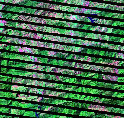
| 9 Feb 2011 image | 9 Feb image filled with 25 Feb 2011 image | ||
 |
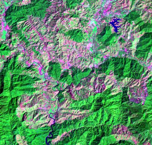 |
This document describes how to apply this gap filling technique using an add-on module in the ENVI software. Guidelines are provided for the selection of images that may produce a quality gap-filled Landsat ETM image. Below you can see an example of this gap-filling technique as applied to a pair of Landsat ETM images from Path 130 Row 45 acquired on 9 and 25 February 2011.
Image Selection
Your first step is to find appropriate images that can be used to produce a quality result. Care must be taken when evaluating images for this technique. At a minimum, these images must be accurately co-registered. Images obtained from the USGS GloVis site in the “GeoTIFF plus Metadata” format have all been terrain corrected so this will not be an issue when using these images. If you obtain images from other sources you will need to co‑register these images before proceeding.
Optimal results will be obtained if both images are free of clouds and shadows, or snow and ice. Generally you should try to find images that have been acquired as close in time as possible. Landsat ETM repeats coverage of an area every 16 days. For some studies you may be able to use images approximately one year apart. This would eliminate any scene variation due to sun angle and distance.
Pay attention to local landscape changes such as plant phenology and harvesting practices. For example, you should not combine images acquired before and after leaf-out in areas with deciduous forests. Also consider major events that may change the landscape, such as tsunamis or hurricanes. You should not use images from before and after a major change event to produce a meaningful gap-filled image.
Preparation
In some cases you may want to perform pre-processing functions such as atmospheric correction or conversion of digital numbers to top-of-atmosphere reflectance on these images. Because these are scene-specific operations they cannot be applied correctly to a blended multi-date image. Any pre-processing functions such as these must be done before using this image gap-fill routine.
Finally, you need to evaluate which image will be the master scene to be filled, and which will be used to fill in the gaps. This is a subjective decision based on your review of the selected scenes. Take the time to view the scenes using different band combinations, perhaps even linking the two scenes.
Image Gap Filling
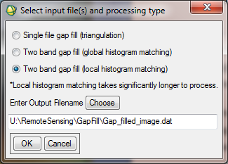 Use the ENVI software program to open the two Landsat ETM images you have selected above. If you are using ENVI Standard interface look under Toolbox | Extensions | landsat_gapfill. If using ENVI Classic, from the main menu bar, select Basic Tools | Preprocessing | Data-Specific Utilities | Landsat TM | Landsat Gapfill. This will open the Select input file(s) and processing type dialog. You should only use the option Two band gap-fill (Local histogram matching), the other options do not perform as well. Next, click on the Choose button to navigate to a folder and enter an output filename.
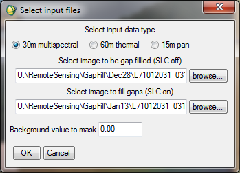 Click OK to open the Select input files dialog box. Make sure you select the appropriate image data type; 30m multispectral, 60m thermal, or 15m pan. Select your master image as the image to be gap filled then select the second image; you will use this to fill gaps in the first image. Click OK and wait for this to complete.
Restore Data Type
The gap-filling technique produces an output image with a 4-byte floating point data type. If you are working with TOA Reflectance values, then your work is complete. However if you are working with the original digital numbers, you should convert these data back to integers. This will reduce the file size by 75% and make all subsequent processing faster.
From the ENVI Classic menu bar, select Basic Tools | Band Math or from the ENVI Standard Toolbox select Band Ratio | Band Math and enter the expression: byte(round(b1))
Click OK and select the button Match Variable to Input File to convert the entire dataset at once. Save this as a new file and delete the gap-filled image created in Section 3 above.
The USGS provides on-demand processing of Landsat 4, 5, and 7 images to create Climate Data Records (CDR)s and Essential Climate Variables (ECV)s. The CDRs are Landsat scenes that have been atmospherically corrected and converted to Surface Reflectance. ECVs are spectral indices derived from the CDRs and include vegetation, moisture and burn ratio indices.
Before ordering these data you should read the USGS CDR Product Guide and/or ECV Product Guide. Data orders are placed using the USGS ESPA Ordering Interface. You will need to provide a text file with a list of desired scenes using the USGS naming conventions. The ESPA User Guide provides information on how to construct and submit an order.
Sentinel 2
Sentinel 2 is part of the Copernicus earth observation program developed by the European Space Agency (ESA) to study the earth’s surface. The Sentinel 2 portion of the program consists of a pair of satellites that are designed to acquire reflected sunlight in the optical wavelengths. It is especially sensitive to variations in vegetation so is extremely useful for studying crops and forests.
Sentinel 2A was launched on 23 June 2015, the first image was acquired on 27 July 2015, and the program became operational on 15 October 2015. The satellite orbits the earth at an altitude of 786 km and has a swatch width of 290 km. This provides a return time of 10 days as compared with the 16-day return time of the Landsat program. Sentinel 2B was launched on 7 March 2017, it is positioned 180° from Sentinel 2A. Together, Sentinel 2A and 2B will provide near-global coverage every 5 days, with quicker return times at mid latitudes.
Data are acquired at three spatial resolutions and should be handled as separate files. There are four bands with a 10m spatial resolution. These are in the blue, green, red, and near infrared parts of the electromagnetic spectrum. The second file has six bands with 20m spatial resolution and the third file has three bands with 60m resolution. The wavelengths are described below. Note that four of the 20m bands are in the red edge and near infrared wavelengths.
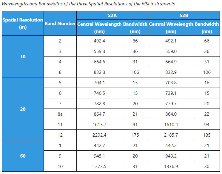
From https://earth.esa.int/web/sentinel/missions/sentinel-2/instrument-payload/resolution-and-swath
Learn more about this program at:
the ESA Sentinel 2 website https://earth.esa.int/web/sentinel/missions/sentinel-2
and the USGS site: https://eros.usgs.gov/sentinel-2
You can obtain Sentinel 2 data from the ESA and from the USGS. Users must register for free access to data at either site. Currently ESA distributes Sentinel 2 data in entire swaths. These files are very large, sometimes 7+ GB when compressed. You can access these data directly from the ESA Copernicus Open Access hub at: https://scihub.copernicus.eu/ Users should read the online User Guide prior to searching for data.
Recommended Site:
The USGS distributes most of the Sentinel 2 data but has cut these data into much smaller tiles of 100 km X 100 km in the Level-1C top of atmosphere reflectance. These data are much easier to work with and users are encouraged to look for data here first. You can access these data at the USGS Earth Explorer site at: https://earthexplorer.usgs.gov/
You should begin your data search by first defining a small region of interest. You can expand this later as needed. You can enter a start and stop date to further limit your search. Next in the Data Sets tab scroll down and select Sentinel | Sentinel 2.
Click on the Results tab to display data that meets your search criteria. You can click on the Footprint icon to show the scene coverage. To the right of this is a Browse icon. This will display the image to help you decide if the scene meets your needs. Users are encouraged to only download one or two images initially. Once you gain experience working with these data you can come back and get more.
These instructions are for those using ENVI version 5.6.1.
Sentinel 2 data use very long folder and filenames that may cause problems in the Windows operating system. You should extract (unzip) the data into a folder near the top of the file structure. By this we mean U:\ rather than something like: U:\Project\Rasters\Sentinel\MyNewData\ImageDate. Once the data are extracted rename the new data folder to a shorter name. Sentinel 2 file name usually takes this fomat:
MMM_MSIXXX_YYYYMMDDHHMMSS_Nxxyy_ROOO_Txxxxx_<Product Discriminator>.SAFE
For example, a Sentinel data folder name might be:
S2A_MSIL1C_20211019T154251_N0301_R011_T18TXL_20211019T192902.SAFE
Which reflects the following infomration: an image obtained via Sentinel 2A (S2A), processed at Level L1C (MSIL1C), acquired on the 19th day of October of 2021 at 3:42:51 PM UTM (20211019T154251), processed with PDGS processing baseline 03.01 (N0301), Relative Orbit Number 011 (R011), Tile Number 18TXL (T18TXL), and its Product Discriminator is 20211019T192902. SAFE is the product format which stands for Standard Archive Format for Europe.
You can rename this file to something like: October19_2021.
To open the image, go the main ENVI menu and select File | Open As | Optical Sensors | European Space Agency | Sentinel 2. Navigate into the new folder and select the XML file. This, however, will be shorter filename such as:
MTD_MSIL2A.xml
ENVI should open the data into files based on spatial resolution. You can examine the data and save the file to ENVI format if you wish to use these data in the future. From the ENVI main menu select File | Save As | Save As… (ENVI, NITF, TIFF, DTED) and follow the instructions to save this file to a new folder structure for your project; it should not be placed in any of the original Sentinel folders. Consider including 10m or 20m as part of the filename to distinguish the resolution.
You can also open these data using the ESA Sentinel-2 Toolbox program SNAP. This is installed on the YCEO Lab systems. You can also download this software from the ESA site:
https://sentinel.esa.int/web/sentinel/toolboxes/sentinel-2
The ESA website has links to documentation and YouTube videos to instruct users. While you can view and manipulate these data quite easily in SNAP, it is a bit difficult to export these data into a format that can be used by ENVI. In order to export these data, they must all have a common spatial resolution. So if you want to use the four 10-meter bands you must resample the entire file to 10 meters. (this is a very large file!) You can then open this in ENVI and spectrally subset this to extract just the four bands of interest.
MODIS
MODIS is an extensive program using sensors on two satellites that each provide complete daily coverage of the earth. The data have a variety of resolutions; spectral, spatial and temporal. Because the MODIS sensor is carried on both the Terra and Aqua satellites, it is generally possible to obtain images in the morning (Terra) and the afternoon (Aqua) for any particular location. Night time data are also available in the thermal range of the spectrum. You should consider time of day when ordering a scene for a specific day.
The MODIS web site, http://modis.gsfc.nasa.gov/index.php, is a good place to begin learning about this important program. This site has links to the Atmospheres, Land and Oceans groups of MODIS. Place your cursor over the Data tab and you can directly access many of the MODIS products.
MODIS data can be placed in two broad categories; daily scenes and derived products. You can order a daily scene for any specific date and location; and at different times of day and night as mentioned above.
Many consolidated products have been developed from MODIS data. These include 8‑day and 16‑day composite images, a variety of indices, and a range of global products with varying time scales. Products are separated into four science discipline groups. Data for each group may be obtained from specific sites and have unique import techniques described below. You can learn about each group at the following sites:
- Land product information can be found at: https://lpdaac.usgs.gov/dataset_discovery/modis/modis_products_table.
- Atmosphere product descriptions can be found at
http://modis-atmos.gsfc.nasa.gov/products.html - Ocean data can be found at:
http://oceancolor.gsfc.nasa.gov/. - Cryosphere data and descriptions are at the National Snow and Ice Data Center
http://nsidc.org/daac/modis/index.html
Next you need to decide where and when you want data coverage. Locations for full daily scenes and products can be entered using latitude and longitude. If you do not know this information, you could use sites such as Google Earth to locate your area of interest and read the coordinates displayed on the screen. Level 2 processed MODIS data such as the Surface Reflectance products are segmented into tiles with an area of 10º X 10º using a sinusoidal projection. Level 3 products are “gridded” into global datasets.
Dates are in the Julian format, i.e. yyyyddd. There is a Julian Date Converter program on the desktops of the YCEO workstations. Time is in Universal Time Coordinated (UTC). The data are provided in the HDF-EOS format.
Daily MODIS Scenes – Level 1
Individual daily MODIS scenes, MODIS Level 1 products, can be obtained for any part of the earth, every day, since February 2000. These files are in the Geographic projection. A complete dataset has a spatial resolution of 1 km and there are 36 bands of data. The data are distributed as digital numbers in 16 bit unsigned integer format. These data should be converted to radiance values, surface reflectance values, and/or brightness/temperature values before performing any analysis.
Terra file names for a complete file begin with MOD021KM. Aqua file names begin with MYD021KM. The product name on the MODIS ordering site is:
“MODIS/Terra Calibrated Radiances 5-Min L1B Swath 1KM V005”.
In addition you can obtain daily scenes at higher spatial, but lower spectral, resolution. Files with 500m resolution contain the 7 bands of data in the Visible, Near-IR and Mid-IR parts of the spectrum. Files with 250m resolution contain two bands of data in the Red and Near-IR parts of the spectrum. The Terra names for these are MOD02HKM and MOD02QKM respectively.
MODIS Products - Level 2
As mentioned earlier, many products have been developed from MODIS data. You should read the product descriptions for each product you intend to use. This will provide information about data range, scaling values, fill values, data type and format, etc. Product data are generally provided in the sinusoidal projection. Below are short descriptions of the surface reflectance and vegetation products. Many more products are available. While the information below is accurate at the time of writing, you should always read the online USGS metadata for any product you plan to work with.
MODIS Products - Level 3
These MODIS data are gridded into global datasets. You can search for these data at the same sites that MODIS Level 2 products are distributed.
Surface Reflectance Products
The surface reflectance products are generated from the first two, or seven, bands of the corresponding full 36 band scenes. These provide an estimated “at surface” spectral reflectance. Several algorithms are applied to various MODIS bands to remove the effects of cirrus clouds, water vapor, aerosols and atmospheric gases. Global surface reflectance products can be obtained at either 250m with 2 bands or 500m with 7 bands, as daily or 8-day composite images.
The data type is 16 bit signed integer, which has a theoretical range of values from -32,768 to +32,768. The documented data range is from -100 to +16000 with a fill value of -28,672. If you wish to convert these numbers to a valid reflectance data range, cell values should be divided by 10,000. These data must then be stored with a floating point data type.
The data are provided in the HDF-EOS format. MODIS data at version 4 and above use the Sinusoidal projection with the WGS84 datum. A very small sample of common products are listed below.
MOD09GQ - MODIS Surface Reflectance Daily L2G Global 250m
This file has a spatial resolution of 250 m and contains two bands of spectral data centered at 645 nm and 858 nm. There are also three bands of additional information on band quality, orbit and coverage, and number of observations.
MOD09GA - MODIS Surface Reflectance Daily L2G Global 500m
This file has a spatial resolution of 500 m and contains seven bands of spectral data plus three bands of additional information on band quality, orbit and coverage, and number of observations. The spectral range for each band can be found in Appendix A, bands 1 through 7.
MOD09Q1 - MODIS Surface Reflectance 8-Day L3 Global 250m
This file is a composite using eight consecutive daily 250 m images. The “best” observation during each eight day period, for every cell in the image, is retained. This helps reduce or eliminate clouds from a scene. The file contains the same spectral information as the daily file listed above, centered at 645 nm and 858 nm. There is one additional band of data for quality control.
MOD09A1 - MODIS Surface Reflectance 8-Day L3 Global 500m
This file is a composite using eight consecutive daily 500 m images. The “best” observation during each eight day period, for every cell in the image, is retained. This helps reduce or eliminate clouds from a scene. The file contains the same seven spectral bands of data as the daily file listed above. It also has an additional 6 bands of information concerning quality control, solar zenith, view zenith, relative azimuth, surface reflectance 500 m state flags, and surface reflectance day of year.
Vegetation Index Products
There are several composite MODIS vegetation products. Sixteen-day composites are available at 250 m, 500 m, 1 km, and 0.05 degree resolutions. There are also monthly composites with 1 km, and 0.05 degree resolutions. Each file contains bands of data for both the traditional Normalized Difference Vegetation Index (NDVI) and Enhanced Vegetation Index (EVI). There are also data quality bands in each file.
The data type is 16 bit signed integer, which has a theoretical range of values from -32,768 to +32,768. The documented data range is from -2000 to +10000 with a fill value of -3000. If you wish to convert these numbers to the traditional data range, cell values should be divided by 10,000. These data must then be stored with a float data type of IEEE 4 byte real.
The Vegetation Index products have a label prefix of MOD13 for the Terra sensor and MYD13 for the Aqua sensor. On the ordering web page the product name indicates the sensor, composite period, spatial resolution, and data version number. For example, “MODIS/TERRA Vegetation Indices 16-day L3 Global 250m Sin Grid V005” will get you the data from Terra for a 16-day composite at 250 m resolution in the sinusoidal projection using the version 5 data
The USGS has a very good collection of videos on YouTube about their various products. The best place to start is to view the short intro to version 6 data. You will learn about the various products, where to find data, how to use the LP DAAC site.
This first introductory video will be followed by more in-depth videos of various products. These are their “Getting Started with…” videos covering Surface Reflectance, Temperature, Vegetation Indexes, etc.
Individual daily MODIS scenes can be obtained at the Level 1 and Atmosphere Archive and Distribution System (LAADS) at: https://ladsweb.nascom.nasa.gov/search/. The page should open with the 1 Products tab active. In the upper left specify the appropriate sensor(s); Terra, Aqua, or Combined. Then select the MODIS Collection. Currently the most recent is Collection 6.
Below this look for the section Level-0 / Level-1 and click on MODIS Terra, Aqua. This brings up a list of MODIS daily scenes on the right. Select the Level 1B Calibrated Radiances dataset at the spatial resolution you wish.
Click on the 2 Time tab and enter a single date or date range. Normally for Coverage Selection you will select only Day.
Next click on 3 Location and use one of the methods to define your region of interest.
Finally click on 4 Files to make a final image selection.
View the browse images of the datasets that meet your search criteria. After you select the dataset(s) you need, lick the Get Data icon on the bottom toolbar to download your image(s).
While ENVI can import these data directly, you are encouraged to use the MODIS Conversion Tool Kit. Information on it’s use can be found here. If you are working with a 1km file you should process the optical and emissive bands separately; convert the optical bands to Reflectances or convert the emissive bands to Brightness Temperatures. If you do not wish to use the MODIS Conversion Tool Kit then follow the guidelines below.
When working with the MODIS daily scenes you will typically be interested in the Reflectance file and, if you have the 1km resolution dataset, the Brightness Temperature (Emissivity) file. ENVI will convert the provided digital numbers to reflectance or temperature values for you. You must then georeference the dataset to the “Geographic” projection.
- ENVI Standard version 5.2 and all versions of ENVI Classic can easily open and georeference MODIS daily scenes. Instructions for doing this are provided below.
- For ENVI Standard version 5.1 and earlier, and for images that cross the International Date Line, you should use the mctk extension module to ENVI. Check the separate YCEO FAQ for instructions on using the MODIS Conversion Tool Kit.
- Note that as of version 5.2.1 ENVI no longer converts emissivity values to brightness temperature. Users wishing to work with brightness temperature are encouraged to use the MODIS Conversion Tool Kit. Information on it’s use can be found here.
Using ENVI Standard version 5.2
Open a MODIS HDF file from the ENVI main menu File | Open As | EOS | MODIS. The reflectance file is loaded into the Layer Manager and all files are shown in the Data Manager. This includes files for Latitude, Longitude, and Quality. If you get the error message “IDLNARASTER::GETPROPERTY” simply click OK. Explore the scene and examine various band combinations but note that the cell values may not be converted to Reflectance until you save the file when you georeference the image.
From the Toolbox select Geometric Correction | Reproject GLT with Bowtie Correction. Select the input data file you want to work with. Since the File Selection window does not distinguish the types of data, you may need to look at the layer positions in the Data Manager to see if Reflectance is the first, second, or third file in the layer stack.
Click OK and the Reproject GLT with Bowtie Correction dialog window opens. You should change the Interpolation Method to Nearest Neighbor and uncheck Display result. Enter an output file name and location, click OK and wait for the process to complete. When this is done remove the original file from the Layer Manager and load the newly converted and projected MODIS daily scene!
Using ENVI Classic
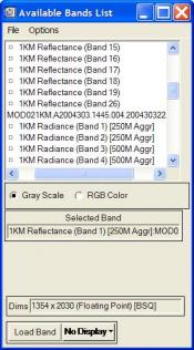 You can use all versions of ENVI Classic to open a MODIS daily scene. From the main menu select File | Open Image File and select your dataset. ENVI automatically converts digital numbers to surface reflectance, radiance, and brightness/ temperature when it opens a full “one kilometer” daily scene. You will see three separate listings in the “Available Bands List” window; identified by band name as Reflectance, Radiance, and Emissive respectively. There will also be one file named Latitude and one Longitude that you can ignore. You typically will only be interested in Reflectance and Temperature (Emissivity) datasets. There will be no data layer for brightness/temperature if using 250m or 500m files.
Initially these files do not display coordinate information, but ENVI can easily generate this. From the main menu select Map | Georeference MODIS. Select a file, click on the “Spectral Subset” button if you wish to use only a few bands of data, and click OK. In the Georeference MODIS Parameters window select the desired output map projection and datum and click OK again. Finally in the Registration Parameters window select a folder and enter a new filename.
Note: ENVI may select the UTM projection by default. Typically these datasets cover an area much larger than a single UTM zone so you should select the Geographic projection and click OK. You can spatially subset and reproject the image later if desired.
When the georeferencing is complete ENVI places a new file with the prefix “Warp” in the Available Bands List. Double click the globe icon to display the coordinate information for this scene. You can view this in a display window and confirm the coordinate information using the Cursor Location/Value tool.
Land Products
A selection of Land products are available at the LAADS site described above in the Daily scenes section. For a more complete collection of MODIS Land products you should search for data at either the GloVIS or Earth Explorer USGS sites or the NASA Earthdata Search site. Each site has a full collection of MODIS Land products along with different collections of other data. They each have a unique interface so the method of identifying the data you desire is a bit different. In each case you will select a location, a product, and a date of interest. You need to create a free account at each site to obtain data.
The USGS GloVis site provides an easy, visual display of each tile to help you select your data. First use the image window in the upper left to navigate to your area of interest and then use the Collections tab to select the MODIS product you want. Once you select the data, click the Add button to place it in your “shopping” cart. When finished selecting data, place the order and you will receive emails confirming the order then providing a link to the data. This is a quick process.
Navigate the USGS Earth Explorer site using tabs along the upper left. Under the Search Criteria tab you are offered several methods to locate your site of interest. You can click a point on the map, manually enter coordinates, or upload a KML or shapefile. From this same screen you can filter the data by time. Next select the Data Sets tab and enter MODIS in the Search box or click on the NASA LPDAAC Collections set to locate your specific data. Click on the Results tab to perform the search and view your results. You can add image footprints to the map and view browse images to help refine your search. You can then immediately download the dataset(s) you wish.
The NASA Earthdata Search site has a good tutorial to help you get started. This will help you easily locate the specific data you need for your project.
Atmosphere Products
NASA has a good site describing MODIS atmospheric products, data formats, content, etc. Your first step should be to review this site:
http://modis-atmos.gsfc.nasa.gov/MOD04_L2/index.html
You can obtain MODIS Atmosphere products from the same LAADS site that MODIS Daily scenes are distributed at: http://ladsweb.nascom.nasa.gov/data/search.html. You should follow the same navigation and search procedures as described in that FAQ, only under Group select Atmosphere Level 2 or Level 3 Products.
Ocean Products
Ocean products have been derived from MODIS, SeaWIFS, and other sensors and are available at the NASA OceanColor site. You should read the descriptions of the products and processing levels before working with these data.
Cryosphere Products
The National Snow & Ice Data Center (NSIDC) is the site to learn about MODIS snow and ice products. They have definitive data descriptions and links to data sources. As with other types of data, please read the data descriptions before downloading any data.
ENVI can open and process most MODIS HDF data. However, the data formats and specific processing steps differ for daily scenes and the various domain products. Daily scenes have geographic coordinate information embedded in the file. Instructions for importing these data are covered in another FAQ. MODIS products are typically distributed using the sinusoidal projection in 10º tiles. Instructions for processing several types of data are described below.
MODIS Land Products
The MODIS Land product data are provided in HDF format using a sinusoidal projection. We recommend using the MODIS Conversion Tool Kit to import these data and reproject to Geographic Lat/Lon if desired as described in another YCEO FAQ.
You can open these directly in ENVI Standard from File | Open As | EOS | MODIS or from ENVI Classic File | Open External File | EOS | MODIS. Select the data layer(s) you wish to use and the new file will be in the sinusoidal projection. Methods for converting the data to the “geographic” projection vary by software version, as described below.
For ENVI Standard version 5.2 in the Toolbox select Raster Management | Reproject Raster. This opens the Reproject Raster dialog window. Browse to the input dataset, then select the Output Coordinate System (Geographic | World | WGS 1984) and finally enter an output filename and click OK.
For ENVI versions 5.1 and earlier you should use ENVI Classic to reproject these data. From the Classic main menu select Map | Convert Map Projection. Another alternative is to use an extension module to ENVI. We recommend using the MODIS Conversion Tool Kit to import these data. This is described in another YCEO FAQ.
MODIS Atmosphere Products
MODIS Atmosphere products are distributed in HDF format as are the Land products. ENVI Standard can open this dataset from File | Open As | EOS | MODIS but it only accesses the reflectance and coordinate files. To access the atmospheric products such as optical depth you are strongly encouraged to open these files using the MODIS Conversion Tool Kit described in another YCEO FAQ.
MODIS Ocean Products
MODIS Ocean products can be opened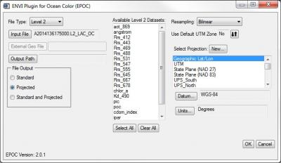 easily in ENVI Standard using the special extension EPOC found in the Toolbox under Extensions. Select the appropriate File Type (Processing Level 1, 2 or 3). Next select the input file and define the output location. For Level 2 or 3 products, choose the appropriate dataset(s) from the available list. Under File Output choose Projected and select the projection Geographic Lat/Lon and click OK to import the new file.
The ENVI Plugin for Ocean Color (EPOC) for ENVI was developed by Devin White. He has graciously made them publicly available on GitHub at: https://github.com/dawhite/ENVIPlugins
MODIS Snow and Ice Products
We recommend using the MODIS Conversion Tool Kit to import these data and reproject to geographic as described in another YCEO FAQ.
Alternatively, if you are using ENVI version 5.2 or above you can open these directly in ENVI Standard from File | Open As | EOS | MODIS or from ENVI Classic File | Open External File | EOS | MODIS. Select the data layer(s) you wish to use and the new file will be in the sinusoidal projection. To convert the data to the “geographic” projection, from the Toolbox select Raster Management | Reproject Raster. This opens the Reproject Raster dialog window. Browse to the input dataset, then select the Output Coordinate System (Geographic | World | WGS 1984) and finally enter an output filename and click OK.
If you are using ENVI version 5.1 or earlier, MODIS Snow and Ice products can be opened as generic HDF files in ENVI Standard from File | Open As | Generic | HDF4. However these files will have no projection or coordinate information.
MODIS Conversion Tool Kit
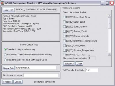 The YCEO Lab uses a plugin module for ENVI to import and convert the projection of many MODIS daily scenes and products in one step. You access the Toolkit from the ENVI Standard interface Toolbox | Extensions | mctk (for ENVI Classic main menu File | Open External File | EOS | MODIS Conversion Toolkit). From the initial Toolkit dialog box click on the Input HDF button and select your file. This opens the expanded Toolkit dialog box.
Under the Processing Options section on the right select the layers of data you wish to import.
Under the Select Output Type section select one of the radio buttons to determine the output coordinate information.
The default, Standard, will retain the sinusoidal tile projection. Selecting Projected will result in an expanded dataset in Geographic projection. You normally would NOT select the third option Both.
Finally enter a Rootname and Output Path for the new dataset.
If you plan to mosaic adjacent tiles you should use the Standard (sinusoidal) Output Type. These sinusoidal tiles can be perfectly joined, whereas the projected data will have gaps at the edges. Once the tiles are mosaicked you can reproject the single seamless file into the Geographic projection.
The MODIS Conversion Tool Kit is one of several plugins for ENVI developed by Devin White. He has graciously made them publicly available on GitHub at: https://github.com/dawhite/ENVIPlugins
The Oak Ridge National Laboratory distributes global subsets of many MODIS land products. The subsets are spatially limited to a maximum of 200 km X 200 km in size but can cover the entire time of the MODIS program. This is an easy way to obtain a time series of data for you research projects.
The data are available at the ORNL DAAC at:
http://daacmodis.ornl.gov/cgi-bin/MODIS/GLBVIZ_1_Glb/modis_subset_order_global_col5.pl
Begin by entering the scene center coordinates or drag the balloon to your location and click the Continue button. Next select one of the many products available. Note that products beginning with “MOD” are from the Tera sensor and “MYD” are from the Aqua sensor. Next enter the number of kilometers Above and Below (north/south) and Left and Right (east/west) that you want for the spatial coverage and hit the Continue button.
On this third page select the beginning and ending times of your requested series. (You should consider selecting a small temporal subset for initial testing before ordering 400+ layers of data.) You are offered a choice of projections, either MODIS Sinusoidal or Geographic Lat/Lon. You should select the Sinusoidal projection; you can reproject the data to a different coordinate system in ENVI later if necessary. Click on the Review Order button. After reviewing your order you can change parameters or click Create Subset to submit the order. You will get an email when this is completed.
Following the link in the email from ORNL brings you to a page with several charts visualizing the data you have selected. After examining these results, click on the Download Data tab and select the Product GeoTIFF Data link to get your data compressed in a “.tar.gz” file. You can use 7-Zip or another utility to extract the data files for your research. Note that this may result in many more files than you expect. For example, the NDVI/EVI Vegetation Index file consists of 22 datasets for each time period. So an order for a two-year cycle of vegetation indexes will produce 528 separate files.
Finally you need to create a single multi-date file containing all of the desired data layers such as NDVI or Land Surface Temperature, making sure the layers are stacked in date order. This can be done easily using a script written with the ENVI programming interface. The YCEO has developed an script that can perform this task for you. See a member of the YCEO staff for a copy of this ENVI script, along with guidance on how to tailor this for your specific needs and execute the script in the IDL environment.
ENVI has more information about programming in their Help section under Contents | Programming | Programming Guide. Also read the short ENVI Programming FAQ on the YCEO site.
The NASA Application for Extracting and Exploring Analysis Ready Samples (AppEEARS) site allows users to access MODIS and Landsat data for selected point locations without the need to actually download these raster datasets. You can manually enter one or more point locations or upload a file of sites for analysis. On the site you can generate charts and graphs of these data individually or in combination, over various time-scales. After exploring the data you can easily download the data for your location(s) as a CSV file.
There are a large number of MODIS and Web Enabled Landsat Data (WELD) products on the site. Users are encouraged to view this USGS YouTube video to learn more about what the site can do, and how to use it. You can also click on the Help link of the AppEEARS page for a short demo of what the site can do and how to use this.
VIIRS
The Visible Infrared Imaging Radiometer Suite (VIIRS) is an instrument onboard the Suomi National Polar-Orbiting Partnership (S-NPP) spacecraft, which was launched October 28, 2011. The VIIRS instrument follows the legacy of, and improves upon, the measurements made by the NOAA AVHRR and the MODIS instruments on Aqua and Terra. VIIRS observes Earth’s entire surface twice each day, with an equator crossing time of approximately 1:30 a.m. and 1:30 p.m. (local time). At an orbit of 835 km, VIIRS scans a swath that is approximately 3000 km wide, 710 km wider than MODIS, and wide enough to avoid gaps in coverage near the equator (unlike MODIS). The VIIRS instrument collects imagery of the land, atmosphere, oceans, and cryosphere across 22 spectral bands, ranging in wavelengths from 0.41 to 12.5 microns, and at two native spatial resolutions: 375m (I-bands) and 750m (M-bands).
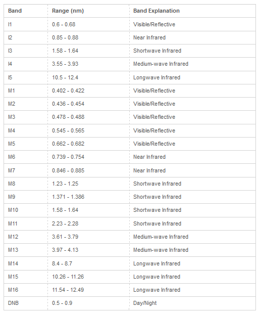
Table source: NASA/USGS LP DAAC
Land data: To allow consistency with MODIS, NASA resamples surface reflectance and other land products (vegetation indices, LAI/FPAR, thermal anomalies and fire) to 500 m, 1 km, and 0.05 degrees. These data are available as daily images, or 8-day to monthly composite images, and distributed as 1200 km x 1200 km tiles in a sinusoidal projection system. For more information, click here. Information for each NASA VIIRS land product can be found in the VIIRS Product Table.
The surface reflectance data are created by applying corrections for atmospheric gases and aerosols to the top of atmosphere reflectance data. Surface reflectance data are available from January 19, 2012 to present. Through LP DAAC, several surface reflectance products are available:
| Refectance product | temporal frequency | spatial resolution |
|---|---|---|
| VNP09GA | Daily | 500 m (I-bands), 1 km (M-bands) |
| VNP09A1 | 8-day composite | 1 km (M-bands) |
| VNP09H1 | 8-day composite | 500 m (I-bands) |
| VNP09CMG | Daily | 5600 m (0.05 degrees) |
In the VIIRS Product Table, you can click on each surface reflectance product to obtain more information and to find links to access the data.
NASA Earthdata Search provides access to surface reflectance data as well as the other NASA VIIRS products.
After creating an account and/or logging in, you may search for the product name (e.g. VNP09A1), as well as define your geographic area of interest and temporal range. The footprint of the VIIRS tile(s) that covers your area of interest will be shown on the map. You can then download some or all of the tiles that meet your criteria, or have them emailed to you.
For first-time users, it is recommended to watch Getting Started with VIIRS Surface Reflectance Data Part 1, which provides a step-by-step guide of finding and downloading VIIRS surface reflectance data from NASA Earthdata Search.
ASTER
The ASTER (Advanced Spaceborne Thermal Emission and Reflection Radiometer) sensor is an imaging instrument flown on the Terra satellite which was launched in December 1999. ASTER has been designed to acquire land surface temperature, emisivity, reflectance, and elevation data and is a cooperative effort between NASA and the Japanese Ministry of Economy, Trade, and Industry (METI). As of April 1, 2016 these date are being distributed free of charge.
You can learn more about the ASTER program at: http://asterweb.jpl.nasa.gov/ or view this hour-long NASA ASTER YouTube video.
This document does not cover the 30m ASTER Global Elevation Dataset. You can find information about the ASTER GDEM data in the DEM FAQ on this site.
An ASTER scene covers an area of approximately 60 km by 60 km and data is acquired simultaneously at three resolutions.
VNIR - 15m spatial resolution - 3 bands at Green, Red, and Near InfraRed wavelengths
- for the AST_L1B dataset only, there is also a backward viewing band 3B.
SWIR - 30m spatial resolution - 6 bands between 1.65 and 2.40 micrometers
TIR - 90m spatial resolution - 5 bands between 8.29 and 11.13 micrometers
Note: Since April 2008 the ASTER SWIR sensor has been subjected to abnormally high temperature abnormalities and these bands should not be used. The VNIR and TIR data are fine.
The images are georeferenced to the WGS-84 datum and Universal Transverse Mercator projection. Data are acquired when tasked and the telescopes on the ASTER sensor can be pointed to each side to expand data collection opportunities. As a result, images do not have regular and repeating path and row footprints as many other sensors have. This can provide a challenge when searching for imagery over time.
As of the spring of 2016 the primary full ASTER individual dataset is the AST_L1T: ASTER Level 1 Precision Terrain Corrected Registered At-Sensor Radiance product. The AST_L1T product has a very high level of geometric correction and the scenes are distributed with a North-Up orientation. All prior ASTER scenes have been reprocessed to this data format. A complete ASTER scene consists of 14 bands of data as described above. In addition you can select full resolution browse images in GeoTIFF format suitable for use in GIS programs along with several Quality Assurance files. You should read the USGS AST_L1T product page for full dataset details.
The earlier ASTER version AST_L1B: ASTER Level 1B Registered Radiance at the Sensor product includes the backward viewing NIR band labeled 3B and is delivered in the along-track orientation. These scenes should be rotated so north is up. This is described in the FAQ Importing ASTER with ENVI.
There are several ASTER products derived from individual scenes such as temperature, emissivity, and reflectance. You can view the full list of products, as well as individual product documentation sheets at: https://lpdaac.usgs.gov/dataset_discovery/aster/aster_products_table. Each product has unique scaling factors and fill values that are described in the product documentation. For example, the AST_08 Surface Kinetic Temperature product has a valid data range from 200 to 3200 and must be multiplied by 0.1 to restore the values to degrees Kelvin.
Note: If you are considering working with the AST_07: ASTER Surface Reflectance VNIR and SWIR product prior to April 2008, you may want to consider using the AST_07XT: ASTER Surface Reflectance VNIR and Crosstalk Corrected SWIR product instead. One SWIR band has defective shielding, leading to light leakage to other SWIR bands. This is referred to as Crosstalk. An algorithm has been developed to remove this aberration.
NASA and the USGS both distribute full ASTER Level 1T scenes for immediate download and allow you to place orders for ASTER products. Examples of ASTER products include Surface Reflectance, Temperature, and Elevation. The full list of ASTER products are described at: https://lpdaac.usgs.gov/dataset_discovery/aster/aster_products_table.
You can download full ASTER L1T scenes from several NASA and USGS sites such as the Earthdata Search Client and Earth Explorer sites.
If you are only interested in full L1T ASTER scenes, the USGS Earth Explorer site is very easy to navigate. Go to the Earth Explorer site, select the Data Set tab, then NASA LPDAAC Collections | ASTER Collections | ASTER Level 1T. Next select the location and time range you are interested in. You can also select the ASTER Global DEM product here.
We have several FAQs to help you search and download these data. Please read these separate ASTER FAQs:
- USGS GloVis FAQ - - L1T and Products
- NASA Earthdata Search FAQ - - L1T (Products soon)
GloVis is the USGS Global Visualization Viewer site that is a primary source of data from many sensors. This FAQ only covers ASTER data. Connect to the site at: http://glovis.usgs.gov/. This will use Java to open a data visualization window (it may be behind your current browser window). Note: You must be a registered user to place orders within GLOVIS.
Navigate to your area of interested by entering the Landsat Path/Row, latitude and longitude in decimal degrees, or use the navigation image sliders and click on a location in the interactive map. You may need to zoom in using the Resolution menu, or pan to your specific location. There are typically many images stacked for each location. You can reduce the list by adjusting the percent of maximum cloud cover.
From the Collection menu select the ASTER L1T Day (VNIR/SWIT/TIR) to search for and obtain Level 1T ASTER scenes. (You can select the ASTER L1T Night collection for night-time temperature data.) If you are searching for an ASTER product, then you must select the ASTER L1A Day (VNIR/SWIT/TIR) from the Collection menu. Later in the Shopping Basket you will select the desired product.
For viewing resolutions greater than 155m, the upper-most scene in the display will have a yellow selection box around it. You can right click on this to bring up a menu of options. These include opening a new window to display a larger browse image or detailed metadata. The Select Scene option lists all available data at the specific cursor location. You can select any one of these to bring it to the top of the stack. Images that you are sure you do not want can be hidden to simplify your selection process.
After finding a desired image; click on the Add button or right click the image and select Add to Scene List. When you are done selecting scenes, click on the Send to Cart button to open the Shopping Basket window.
In the Shopping Basket web page you will use the Select Process button to select any ASTER product, or if you want the basic ASTER scene select ASTER Level L1T. Make sure you have selected the Level 1T data or a product based on the L1A selection; you do NOT want the Level 1A data! If you want multiple products for the same scene, you will need to return to the GLOVIS application, reselect the dataset, add it to the shopping cart, and select the processing level. When all data have been selected submit the order for processing. An email will be sent with a link to retrieve the data.
The NASA Earthdata Search application provides an easy way to find ASTER scenes, including ASTER products. ASTER products have additional processing so you will not be able to immediately download these data. You can enter a simple natural language search term such as “Aster temperature over Connecticut for 2017” or follow the guide below for a more targeted search.
Begin by navigating to the Earthdata Search application and click on the Spatial button and select the tool you wish to use to define your area of interest; this can be a rectangle, point, polygon or file. Once you have defined your spatial location, enter ASTER L1T into the search box in the upper left. The number of granules will be displayed in the center panel. You can click on the Temporal tab to apply a time filter to your search and reduce the number of granules selected.
Now you have identified the Where, What, and When for the data you are searching for. Next, in the middle panel click on the Matching Collection to open the Project Collections panel on the left that displays each scene meeting you search criteria. As you move the mouse over each item the actual scene footprint is displayed. Clicking on a scene lets you view browse images. Click on the X to remove scenes that are outside of your area, have too many clouds., or do not meet your project needs for other reasons.
You can retrieve individual scenes (recommended) from the download icon on each scene or you can click on the Retrieve Collection Data button to order the entire collection you are viewing. This could be a large amount of data so make sure you have removed any low-quality scenes and those on the margins of your study area.
The following instructions describe how to open ASTER data using the ENVI 5.x Standard interface. You can perform the same steps in ENVI Classic under the Basic Tools menu. ASTER data sets and products are distributed in the hierarchical data format (HDF). Use the following method to properly open and calibrate these data in ENVI.
- In ENVI 5.3, from the ENVI menu select File | Open As | Optical Sensors | EOS | ASTER.
- In prior versions of ENVI 5.x, from the ENVI menu select File | Open As | EOS | ASTER.
ASTER scenes contain files with three different spatial resolutions. When you open the HDF file the ENVI software creates up to four virtual files for these data. The first contains three VNIR bands with 15m resolution. The second, for L1B data only, is the backward viewing NIR band, also at 15m resolution and rarely used. The next file contains six SWIR bands at 30m resolution. Note that images acquired after April 2008 do not have the SWIR data. Finally the last file contains the five TIR bands at 90m resolution.
In most cases ASTER products have been scaled before archiving at the USGS. Please read the USGS product documentation to determine if these data must be rescaled, and what is the appropriate value.
ASTER L1B data and ASTER products (as of this writing) are delivered in along track orientation and should be rotated to north-up orientation. This is described in the Image Rotation FAQ on this site.
ENVI automatically applies the proper calibration coefficients to convert the integer digital numbers to floating-point radiance values when opening a Level 1B or 1T dataset. You can easily convert these values to Top-Of-Atmosphere Reflectance in ENVI. From the Toolbox select Radiometric Correction | Radiometric Calibration and select the three-band VNIR file. Change the Calibration Type to Reflectance, enter a new filename, and click OK.
ENVI has a multi-step process that can perform basic atmospheric correction then convert the resulting emissivity bands to a brightness-temperature image in degrees Kelvin. When ENVI reads an ASTER AST_L1B scene it calibrates the TIR bands to proper radiance values. If you are working with one of these datasets proceed to Step 2. For the newer ASTER AST_L1T datasets ENVI opens these with “byte values” which must first be converted to floating-point radiance values as shown in Step 1.
Step 1
From the Toolbox select Radiometric Correction | Radiometric Calibration and select the five-band TIR file. Make sure the Calibration Type is Radiance, enter a new filename, and click OK
Step 2
From the Toolbox select Radiometric Correction | Thermal Atmospheric Correction and select as input the five‑band TIR file for AST_L1B datasets or the file created in Step 1 for AST_L1T datasets. In the dialog window take all defaults and enter an output filename to create the input to the Emissivity Normalization process.
Step 3
Again from the Toolbox, select Radiometric Correction | Emissivity Normalization and select the Thermal Correction file just created in Step 2. Take all defaults, make sure the Output Temperature Image is toggled to Yes and enter a filename for this.
You will now have a brightness temperature file with units in degrees Kelvin. You can convert this to Celsius using band math to subtract 273.15 from the file.
ASTER L1B full scenes and ASTER products (as of this writing) are delivered oriented along the satellite path. While these data are georeferenced, they are NOT oriented with north at the top of the image. These data should be rotated into a map orientation with north being at the top of the image. This step is NOT necessary for ASTER L1T full scenes.
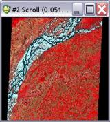
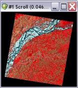
Below are two views of an ASTER dataset illustrating this issue. The left image is aligned to the along-track orientation, the angled path the satellite travels across the face of the earth. The right image has been rotated so north is up.
You should rotate these images to align them so north is up. Prior to performing this you need to check the data values of cells outside of the image, the black or white areas in the margins. This may be something like –NaN or 0 (zero). You will use this value as the background filler value in the next step.
From the Toolbox select Raster Management | Rotate / Flip Data. Accept the default Angle because ENVI extracts the correct rotation angle from the header information. Enter the margin value from above as the new Background value. Then enter a new filename and click OK to rotate the image so that North is Up.
Proba
The Proba-V sensor is a European follow-on to the SPOT VGT mission. It acquires global images of the earth’s land surface and vegetation growth every two days (five days at 100 m resolution). Data are acquired at four wavelengths; blue, red, NIR, at 100 m resolution and SWIR at 200 m resolution. View the Proba-V mission page for more detailed information.
Several products are available and are distributed at 100 m, 300 m and 1 km spatial resolutions. The 1 km products are freely available to all users as soon as they are compiled. The 100 m and 300 m products are freely available one month after they are compiled.
You can view a nice collection of images at the Proba-V gallery. The images are thematically organized and show the capabilities of these data.
This FAQ describes the types of Proba-V products available for free download
Proba-V products are organized into Collections by spatial resolution, number of days for a composite, and processing level. The data are distributed in 10° x 10° tiles in the HD5 format.
Collections with an S1 designation are composite images made up from the best pixels for that particular day. S10 collections are composite images made up from the best pixels over a 10 day period. The S5 collections are 5-day composites of the 100 m data only.
Collections are further subdivided by processing level. TOA represents Top Of Atmosphere reflectance data. The TOC collections are made from the TOA collection with atmospheric corrections applied to the data. These collections include the VNIR (Blue, Red, NIR) bands and SWIR and NDVI layers. There is also a 10-day composite with just the NDVI layer. For example, the collection S1 TOC - 300 m contains one-day composite data that have been atmospherically corrected and contains five bands of data at 300 m spatial resolution.
These data can be downloaded ESA VITO Product Distribution Portal. You must register as a user (free) to download data. Click on the Collection to bring up the product search page. Once you are familiar with the tile designations you can more directly access data via the Fast HTTP Access link.
ENVI version 5.2 software can open the S1 and S10 collection HD5 files directly. When you open a multispectral HD5 file ENVI will create an RGB layer displaying the NIR, Red, and Blue layers respectively. Data are automatically scaled to reflectance values. The SWIR band and NDVI band are placed in the Data Manager as separate files and can be displayed from there.
At this time ENVI cannot open the S5 100 m collections in HD5 format. When you download these data you should select the TIFF option. You must then divide the data by 2000.0 to convert the data into reflectance values.
DEM
Digital elevation data can now be obtained for any place on the Earth, at several resolutions. This document will discuss the major sources for reliable and freely available DEM data. In order to choose the right source for DEM data, there are two main criteria to consider: geographical region of interest and spatial resolution. Below is a table that summarizes the DEM data sources that should be of interest to you.
|
Source Type |
Geographical Region |
Spatial Resolution |
Notes |
Source Link |
|
U.S., Puerto Rico, Territorial Islands of the U.S., and Mexico |
1 arc-second (30 m) 1/3 arc-second (10 m) 1/9 arc-second (3 m) 2-arc-second (60 m) – only Alaska |
Most preferred for continental U.S. |
||
|
Global Global U.S. |
3 arc-second (90 m) 1 arc-second global 1 arc-second for U.S. |
Version 2: finished Version 3: Void fill Version 3 |
USGS Earth Explorer
Reverb | Echo |
|
|
Global |
1 arc-second (30 m) |
Only between 83ºN and 83 ºS |
USGS Earth Explorer |
|
|
Global Multi-resolution Terrain Elevation Data 2010 (GMTED2010) |
Global |
30 arc-second (1 km) 15 arc-second (450 m) 7.5 arc-second (225 m) |
Replaced GTOPO30, preferred for working with very large regions |
USGS Earth Explorer |
The National Map is the primary source of the National Elevation Dataset (NED) data of the U.S. at: http://nationalmap.gov/viewer.html.. When you first visit this site you should read the directions for downloading data from the National Map Viewer before searching for data. This will teach you to easily navigate the site and select exactly what you need. These data have a Geographic “projection” (latitude/longitude) and use the NAD83 datum. You will find that there are many other types of data available at this site. You should explore this site at your convenience.
Within the U.S. you can access NED data at 1 arc second (~30 m), 1/3-arc-second (~10 m), and in some locations 1/9-arc-second (~3m) resolution. For Alaska, the NED data are primarily 2-arc-second (~60 meters). All of the data are prepackaged in 1x1 degree tiles, except for 1/9 arc second data that are prepackaged in 15x15 minute tiles.
Zoom in to your area of interest and click on the Elevation Availability in the Table of Contents on the left. If a certain checkbox is disabled or an error notification box appears, then zoom in for finer spatial resolution. Reminder: the data is available for only North America (U.S., some Canada, and Mexico).
Once you have confirmed the dataset you are interested in is available, click on the Download Data button on the toolbar or in the upper right of the window. There are a few options for defining your region of interest; draw a rectangle; select a reference area, adjust current map extent, or enter coordinate input. Select a method then specify the type of data you would like to download, in this case Elevation, and click Next.
You are presented with a list of tiles at different resolutions, in different formats. Currently the output formats available on the National Map Viewer are IMG, ArcGrid, and GridFloat. You should choose the IMG format if working with ENVI.
Check off the product(s) you are most interested in and click Next. The Table of Contents pane changes to a view of your Cart. Check out by providing your email address. The link (or multiple links depending on the size of the region) to download the data will be sent immediately to your email address.
In February of 2000 the Space Shuttle mapped most of the land surfaces of the Earth, from 60° north to 56° south, to create the highest resolution global elevation dataset available to date. Global data were released at a 3 arc-second (~90 m) resolution. Data covering the United States were also released at a 1 arc-second (~30 m) resolution. The Version 1 data had many data voids and irregular water surfaces and coastlines.
Version 2 SRTM Data
NASA released a “finished” version of these data called Version 2. These data had most voids filled in by interpolation, lake surfaces were corrected, and coastlines properly defined and aligned. These data are available at the USGS Earth Explorer site. Data are available at 3 arc-second (~90 m) resolution globally, and also at 1 arc‑second (~30 m) in the U.S. Care should be taken when using SRTM data in areas with extreme topographical change as there are still data voids in some of these areas.
Version 3 SRTM Data
In November 2013 NASA released Version 3 of the SRTM data. These data had voids filled using other data sources such as the ASTER GDEM2, GMTED2010, and NED. These are the highest quality SRTM data available to date. Get these data at the NASA Reverb | Echo site. As with the Version 2 data on the USGS site, these data are available at 3 arc-second (90 m) resolution globally, and also at 1 arc‑second (30 m) in the U.S. and most of the world.
To obtain these data on the Reverb site zoom in to your area of interest then enter the keyword SRTM in the Search Term box in the upper right. Under Step 2: Select Datasets select the V003 dataset you wish, either NASA Shuttle Radar Topography Mission Global 3 arc second V003 or NASA Shuttle Radar Topography Mission Global 3 arc second V003, then click Search for Granules. (Do not select the datasets that have the phrase “second number V003” as part of their tittle.) Data are packaged in 1° x 1° tiles. Use the Browse button to view the granule(s) and put those you want into your Cart. From the Cart click on the Download button and a text file will be generated that can be used to download your data. Simply paste this line of text into your browser to get the data.
These integer data use the Geographic “projection” (latitude/longitude) and the datum is WGS84. The data are in “height” format with a file extension of .HGT. To open these data in ENVI Standard, from the main menu select File | Open As | Digital Elevation | SRTM DEM.
Global 1 Arc-Second Data - best choice for 30 m resolution
Beginning in September of 2014 the USGS began distributing 1 arc-second Version 3 void-filled data globally. Unlike the original Version 3 release, these data will be distributed through the USGS Earth Explorer site. Click on the Data Sets tab then Digital Elevation | SRTM. Data are packaged in 1° x 1° tiles and distributed in three formats; DTED, BIL, and GeoTIFF. GeoTIFF data may be the easiest to use in most geospatial software programs and is the recommended format.
The science teams at the NASA Jet Propulsion Lab (JPL) and Japan’s Ministry of Economy, Trade, and Industry (METI) used the ASTER sensor onboard the Terra satellite to produce 30 m resolution elevation data. These data cover 99% of the land surface from 83° north latitude to 83° south latitude. Version 2 of these data was released in October 2011 and is a significant improvement over the initial data release. You can view the latest information about these data at the USGS LP DAAC
These ASTER data are now available at the USGS Earth Explorer site. You may zoom in, create polygon features, or enter path/row information to select your area of interest. Then select Digital Elevation, then ASTER GLOBAL DEM, and click Results.
These data may be packaged in many tiles. You can turn on or off individual tile footprints and immediately download each tile. If there are many tiles you can select them for Bulk Download, which will add the results to your “shopping cart.” You will receive an email when the data are available for retrieval and you then use the USGS Bulk Download Application (installed on the YCEO Lab computers) to easily retrieve your data.
The USGS has global DEM data at several resolution levels: 30-arc-second (1 kilometer), 15-arc-second (450 meters), and 7.5-arc-second (225 meters). The GMTED2010 dataset with multiple resolution levels replaces a former version called GTOPO30, which only had the resolution level of 30-arc-second (1 kilometer). These data have been collected from a variety of sources using aggregation methods. These datasets are best used for working at the continental scale and with very large regions. More information is available in the USGS publication.
The data can be accessed via the Earth Explorer site. First define your region of interest under the Search Criteria tab. You can upload a Shapefile (in Lat/lon), a KML file, or use the view window extents. Next select the Data Sets tab and under Digital Elevation select GMTED2010. Click on the Results button at the bottom of the screen and data that meets your selection is placed in the Results tab.
Click on the Footprint icon to view the size of the tile. These cover a very large area. Click on the Download icon and you can select the DEM resolution; 7.5 Arc Sec (225m), 15 Arc Sec (450m), and 30 Arc Sec (1km).
These integer data use the Geographic “projection” (latitude/longitude), the datum is WGS84, and are provided in TIF format. There are seven products in each order including min, max, mean, and standard deviation. For most applications you will use the Mean identified with “gmted_mea” in the filename. More information about these different products can be found in the USGS document referenced in the first paragraph.
A copy of the global 30-arc-second (1 kilometer) GMTED2010 data has been downloaded for internal use to a server at the Yale Center for Earth Observation (YCEO). Please see a member of the YCEO staff for guidance in using these data.
ENVI Standard version 5.1 and above also has the 30-arc-second (1 kilometer) GMTED2010 dataset embedded into the application. Access these data from ENVI; select File | Open World Data | Elevation (GMTED2010). As of January 2016 ENVI software on the workstations in the YCEO Lab provide the 7.5 Arc Sec (~225m) GMTED2010 dataset in JPEG 2000 format.
Land Cover
The MODIS Land Cover Type product is a global land cover classification data layer produced annually from 2001 through 2013 (as of this writing). For each year there are five land cover schemes, developed by different research groups. Data are distributed by the USGS at 500m resolution in standard MODIS grid tiles. These tiles use the sinusoidal projection and cover approximately 1200 x 1200 km (~10° x 10° at the equator). The following USGS site has detailed meta data and download access:
https://lpdaac.usgs.gov/dataset_discovery/modis/modis_products_table/mcd12q1
The MODIS Terra + Aqua Land Cover Type Yearly L3 Global 500 m SIN Grid product incorporates the following five different land cover classification schemes, each derived through a supervised decision-tree classification method:
Land Cover Type 1: IGBP global vegetation classification scheme
Land Cover Type 2: University of Maryland (UMD) scheme
Land Cover Type 3: MODIS-derived LAI/fPAR scheme
Land Cover Type 4: MODIS-derived Net Primary Production (NPP) scheme
Land Cover Type 5: Plant Functional Type (PFT) scheme
The five research groups developed their own classification schemes to categorize land cover properties using one year of Terra and Aqua MODIS data. The International Geosphere Biosphere Programme (IGBP) Type 1 land cover scheme identifies 17 land cover classes (0 – 16) which includes 11 natural vegetation classes, 3 developed and mosaicked land classes, and three non-vegetated land classes. Information about all of the data layers, including Quality Control are shown below. Also the categories and class codes for the five classification schemes are listed.
Basic File Information
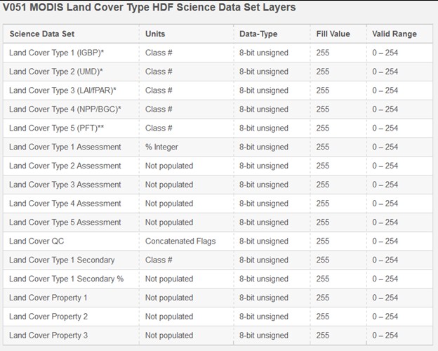
Classification Schemes 1 - 4
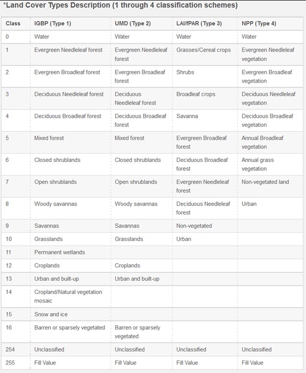
Classification Scheme 5
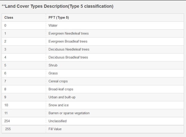
Friedl, M. A., Sulla-Menashe, D., Tan, B., Schneider, A., Ramankutty, N., Sibley, A., andHuang, X. (2010). MODIS Collection 5 global land cover: Algorithm refinements and characterization of new datasets. Remote Sensing of Environment, 114, 168–182.
Obtain the land cover data for the location and year(s) that you are interested in from the USGS site:
https://lpdaac.usgs.gov/dataset_discovery/modis/modis_products_table/mcd12q1
Data are distributed in the Hierarchical Data Format (HDF) and each file contains multiple layers of data. While you can open this file directly in ENVI, this will not retain any coordinate information. You should use the MODIS Conversion Tool Kit (MCTK) found under the Toolbox | Extension | MCTK.
Select the HDF file then pick the data layer(s) you are interested in. Unless you plan to mosaic multiple tiles, choose Reprojected Rigorous georeferencing under the Select Output Type section. In the right-most panel that opens select Geographic Lat/Lon and enter 255 for the Background Value to Use. Enter an Output Path and Rootname and click the Process button.
When the data are imported ENVI will not recognize this file as a classified image. You can use the ENVI tools to edit the header file but it will be much simpler to modify this with a text editor. Make a backup copy of the ENVI header file that you have just created, the file with the .HDR file extension. Now open the original header file with a text editor and paste the contents of the IGBP-Class-Info.txt file at the end of the header file. Save the header file then use the ENVI Data Manager to close the file. Reopen the file in ENVI and it will be recognized as a classification image, with the appropriate Class names and colors, and the Data Ignore value will be set to 255. You can use this same IGBP Class file for the University of Maryland Type 2 classification scheme.
If you have already imported these data following the MODIS Land Cover data in ArcGIS FAQ you can simply open the TIF file in ENVI. If you used ArcGIS to reproject the raster from sinusoidal to Geographic then ENVI will recognize the coordinate system.
Obtain the land cover data for the location and year(s) that you are interested in from the USGS site:
https://lpdaac.usgs.gov/dataset_discovery/modis/modis_products_table/mcd12q1
Data are distributed in the Hierarchical Data Format (HDF) and each file contains multiple layers of data. Once you have downloaded the MCD12Q1 data for the MODIS tile(s) covering your study area you can open the file in ArcGIS. When you select the HDF file the Subdataset Selection dialog opens. Choose the data layer corresponding to the classification type you want to work with and click OK. There is no need to create a pyramid layer at this time.
The data are displayed as a gray scale image and you cannot adjust the display using the unique land cover class codes. Export this layer as a TIF by right-clicking on the file name then selecting Data | Export Data and selecting the TIFF format when you save the new file. Next you need to build an Attribute Table. Open the Attribute Table for editing and add a new field for the land cover Class names. Enter the Class names for the classification scheme you have selected. These names can be found in the FAQ describing the product.
You should then apply a consistent color scheme to your classification data. Here is an example Color Map designed for the IGBP Type 1 classification layer. Right-click on the link and save the file with a new name MCD12Q1.clr or copy and paste the data into a new file with this name. You can apply this to your TIF by right-clicking on the file in the Table of Contents and selecting Properties | Symbology then click on the Colormap button and import the Color Map. This Color Map can also be used with the Type 2 University of Maryland classification scheme.
These data are in a MODIS sinusoidal projection. You should consider reprojecting the raster dataset to the Geographic WGS84 coordinate system.
The Global Land Cover Characterization (GLCC) dataset is a collection of land cover classification schemes based on AVHRR data from April 1992 through March 1993. These data are available by continent or a single global coverage in either the Interrupted Goode Homolosine projection or in geographic coordinates (latitude/longitude). These data are available at the USGS Earth Explorer site.
You can learn more about the product at the USGS Global Land Cover Characterization site.
Climate
The National Oceanic & Atmospheric Administration (NOAA) has been acquiring and distributing climate and weather data for quite some time. The Physical Sciences Division (PSD) of the NOAA Earth System Research Laboratory (ESRL) is a great course of many forms of data. Here you can find hourly precipitation over the U.S. or the monthly Palmer Drought Severity Index from 1850. Do you want daily Outgoing Longwave Radiation, monthly Soil Moisture from 1948, or Ocean Salinity? How about 2015 Cooling Degree Days Anomaly or last week’s mean Sea Surface Temperature? You get the idea; there is a vast collection of data that is easily accessible to you.
Start your search by navigating to the ESRL – PSD site at: http://www.esrl.noaa.gov/psd/
Take some time to explore the site. Under the Data link look in the Gridded Climate and Satellite sections. Next under the Products link explore the Map Room. You can generate many static or looping maps of Sea Surface Temperature, El Nino events, Outgoing Longwave Radiation and other data. For most data you can generate a nice map and then download the data used to produce this in a format you can use for further analysis!
Search and Plot Data
One of the real highlights of the site is the Plotting & Analysis section under the Products link. There are many links to navigate directly to sub sections of the site. The first link, Search & Plot Data is a very good way to dig into the many forms of data available. Select a Data Set such as NOAA Global Temperature or a Variable such as Wind Speed and click Search. You will be presented with one or more products to explore. Click Create a plot or subset in the product you wish to work with and you are taken to a page to define your plotting terms.
The Axis Dimensions section defines the spatial extent. The Other dimension Value section will allow you to select a temporal range. We recommend a few changes in the Plot output options section to improve data visualization. Change the default Contour Lines to Contour Fill and increase the Scale plot to 150%. Click on the Create Plot or Subset of Data button to visualize your data. If you need to make changes to your selections use the browser back button and adjust the mapping options. When you have what you want click on the FTP the data link below the plot to download the data in the NetCDF format. These data can be opened in a variety of analysis software including ENVI, ArcGIS and Matlab
Techniques
ENVI can calculate the Tasseled Cap Transformation of Landsat MSS, TM, and ETM sensor data. The transforms for each sensor produce a different number of bands. The MSS transform produces a four-band output file with bands identified as: Soil Brightness Index, Green Veg Index, Yellow Stuff Index, and Non-such Index. The TM transform produces a three-band output file with bands identified as: Brightness, Greenness, and Third. The ETM transform produces a six-band output file with bands identified as: Brightness, Greenness, Wetness, Fourth, Fifth, and Sixth. The user is encouraged to consult the literature for assistance interpreting these data.
ENVI, as of version 5.4.1, does not have a function to apply the Tasseled Cap transform for the Landsat OLI (8) sensor. In 2014 Muhammad Hasan Ali Baig and colleagues derived transform coefficients for the Landsat OLI sensor. These coefficients are applied to Landsat OLI bands 2 through 7 (Blue, Green, Red, NIR, SWIR1, and SWIR2) to create new bands identified as: Brightness, Greenness, Wetness, TCT4, TCT5, and TCT6. Below are the published coefficients to produce the Tasseled Cap transformation for the Landsat OLI sensor.
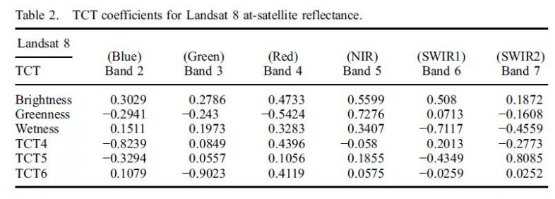
One can use Band Math in ENVI to create new files for the Brightness, Greenness, and Wetness data. If desired, these three new files can be combined into a single file using the Layer Stacking function in ENVI. You can see a member of the Yale Center for Earth Observation for a copy of the ENVI Band Math expressions to produce these new layers of data. They are repeated below for your convenience.
Brightness: b1*0.3029+b2*0.2786+b3*0.4733+b4*0.5599+b5*0.508+b6*0.1872
Greenness: b1*(-0.2941)+b2*(-0.243)+b3*(-0.5424)+b4*0.7276+b5*0.0713+b6*(-0.1608)
Wetness: b1*0.1511+b2*0.1973+b3*0.3283+b4*0.3407+b5*(-0.7117)+b6*(-0.4559)
Note: The new Coastal Blue band 1 of the OLI sensor is not used in these transforms.
Note: Negative values must be enclosed in parenthesis.
Reference:
Muhammad Hasan Ali Baig, Lifu Zhang, Tong Shuai & Qingxi Tong (2014) Derivation of a tasselled cap transformation based on Landsat 8 at-satellite reflectance, Remote Sensing Letters, 5:5, 423-431, DOI: 10.1080/2150704X.2014.915434
To link to the article: http://dx.doi.org/10.1080/2150704X.2014.915434
Often we need to apply the same set of functions to multiple files. For example, you may want to import a collection of Landsat images, apply radiometric calibration to Top of Atmosphere reflectance, and subset the images to your study area. Or perhaps you want to import and stack MODIS day-time Land Surface Temperature (23 per year) for five years. Then repeat this process for the night-time temperatures. These can be done individually in ENVI but may take a lot of time and effort .
The ENVI Application Programming Interface (API) can be used to automate many of these repetitive tasks, performing many steps on a large number of files in a batch mode. These programs (scripts) are based on the IDL programming language and are run in the IDL environment, either by loading the ENVI+IDL program or simply loading IDL by itself. You can manipulate the ENVI GUI via scripts, or run the scripts without even loading ENVI. Please see a member of the EOL staff to learn more.
The ENVI API uses an object-oriented design to operate on data and manipulate the environment. Use the ENVIRaster object to open a file, or the View function to add a new View in the GUI. There are a large number of ENVI Tasks that can be called to perform many operations such as stacking layers, classifying an image, or reprojecting a raster. The API also uses many IDL routines to control looping and other methods of flow control, file searching, directory navigation, etc.
Learn more about programming in the ENVI Help section under Contents | Programming | Programming Guide. This provides a good introduction and a number of examples to help you get started. Harris Geospatial Solutions, ENVI’s parent company, has much more detailed information on their site. Learn about the ENVI Task objects at: https://www.nv5geospatialsoftware.com/docs/ENVITask.html
Detailed function specifications can be found at: https://www.nv5geospatialsoftware.com/docs/routines-2.html
For those wishing to dig even deeper, check out the IDL Programming guide at: https://www.nv5geospatialsoftware.com/docs/idl_programming.html
How to capture Google Earth images for use in ENVI
There are times when you may want to capture high resolution screenshots form Google Earth to use in ENVI software. This could be for background display, ground truthing, or viewing historical imagery. Basically in Google Earth you will navigate to the area you wish to capture and place markers in each corner. After saving the image you will use these corner markers to georeferenced your image in ENVI or ArcMap.
This document is based on information in the UCLA Introduction to GIS page “How To: Add a Google Earth Satellite Image Into ArcMap” located at:
http://gis.yohman.com/up206a/how-tos/how-to-add-a-google-earth-satellite-image-into-arcmap/
Preparing and capturing the Google image
Follow the Google Earth section on the above link for detailed instructions on placing corner markers. We recommend using Google Earth Pro, rather than Google Earth, to capture a higher resolution image. Google Earth Pro is installed on all of the PCs in the YCEO Lab. You may need to enter your email address as the username and the password GEPFREE. When you select File | Save | Save Image three buttons are placed above the image. Click on Map Options to turn off the various map elements. Click on the Resolution button and select Maximum. Finally click on the Save Image button to capture the image.
The UCLA page provides instructions on how to georeference the image using ArcMap. Below are instructions on how to georeference the captured image using ENVI.
Using ENVI
- Open saved image in a new View in ENVI
- From the Toolbox select Geometric Correction | Registration | Registration Image to Map
- Select the RGB bands of image to register
- Increase the resolution to retain more detail: 0.00003513 for example
- Select the Upper Left center point and enter the saved Lon and Lat values
- Click Add Point to save this
- Repeat this step for the three remaining corners
- From GCP Selection dialog
- Options | Warp (Displayed bands or File)
- Use Bi Linear interpolation
- Open a new view and display your image
This image could be saved as a GeoPDF and used on a tablet or phone with the Avenza PDF Maps application.
Once you have created a landcover classification in ENVI you may wish to view or work with these data in ArcGIS. If you include a file extension of “.DAT” as part of the filename you can open this file directly in ArcGIS. For example, you can open the file MyClass.dat in ArcGIS and you will see the classified image with the colors that you have specified.
You need to be aware that this is an 8-bit raster image and does not have the attributes of a vector image in ArcGIS, i.e. you cannot use this for zonal statistics, selection by attribute (class), or clipping and buffering other data. To perform any of these GIS functions you will need to convert the ENVI raster file to an ArcGIS shapefile.
When you use the ENVI Classification Workflow the last step has an option to Export Classification Vectors directly to a shapefile. While this is easy to do; generally we need to perform many classifications, modifying the training regions along the way. Also you may want to perform post classification steps such as combining classes. For these reasons, it is generally better to NOT export the classes at this stage of your analysis.
Once you have performed your image classification(s) and assessed the accuracy of your work, there is a simple two-step process that you can use to convert the final classified raster data into a vector file structure that can be used in ArcGIS. Be advised that this could be a time consuming process on large images with many class polygons.
Export to Vector:
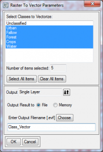 From the ENVI Toolbox select Classification | Post Classification | Classification to Vector. Select your classified image and click OK to open the Raster To Vector Parameters dialog. You have several options within this dialog; you can select all classes or some subset of them, you can save all of the data to a single layer file or save each class as a separate layer.
Typically you will select all classes into a single layer file. Make sure you do not select the default class “Unclassified” or a class labeled “Masked pixels” (created if you applied a mask to your image). Direct the Output to a Single Layer, enter a new filename such as Class_Vector, and click OK. This creates an ENVI vector file with the file extension “. EVF” When opened in the Layer Manager or Data Manager this will display the name RTV(your original classified file name).
Export to Shapefile:
Using the Toolbox select: Vector | Classic EVF to Shapefile. Select the EVF file from the previous step, enter an appropriate filename for the new shapefile, and click OK. ENVI will append the ‘.SHP” file extension to your filename. It may take some time to complete the export, be patient.
Once this is complete, add this shapefile to a map in ArcGIS. Open the Layer Properties and under the Symbology tab select Categories | Unique Values then click on the button Add All Values to display the separate classes. ArcGIS will use the ENVI class names but will use its own color scheme. You can easily change the individual colors and labels here or in the Table of Contents pane.
One important contribution to the understanding of a landscape is the incoming solar radiation, or insolation, that is available at the surface. While one could use the global average of 1366 watts/m2, actual values are generally much lower. On a global scale the controlling variables are the latitude, distance from the sun, and time of year. At the local level elevation, slope and aspect are major factors in determining the amount of energy available. You will need ArcGIS version 9.2 or greater with the Spatial Analysis extension.
The Solar Analyst module in ArcGIS can be used to calculate Watt-Hours/meter2 at the surface at the local scale. Inputs to this process are a digital elevation model (DEM), the latitude of the scene center, and the date and time that you wish to accumulate insolation. You can specify a portion of a day, or a range of days such as a week or month.
For purposes of this document, we will use the Solar Analyst to accumulate the energy striking the surface for the one hour prior to the acquisition of a Landsat image. You could then compare the amount of energy available at the surface, to the brightness-temperature derived from the Landsat thermal band. Alternatively you could adjust the parameters to compare the amount of energy available over a growing season, to the local land cover.
Required inputs
The most important requirement is an accurate, georeferenced DEM dataset. If you do not have one for your study area, use the DEM FAQ on this site to help you locate one. Make note of the scene center latitude. The Solar Analyst module may not determine this automatically when the dataset is opened.
For this example, the other required inputs are the Julian date and the local time of day of image acquisition. As a reminder, the Julian day of year is simply the sequential number from 1 to 365 (or 366 if a leap year). You can use the Julian Data Calendar, on the YCEO Lab workstation desktops, to calculate this. Local time of day is a function of latitude. The Landsat orbit is designed to cross the equator at approximately noon local time. An orbit takes approximately 90 minutes, or 45 minutes from pole to pole. A rough estimate of the local time is fine.
Create new data layers
Begin this process by loading ArcGIS and activating the Spatial Analysis extension if necessary. Add your DEM to the new empty map. Open ArcToolbox and select Spatial Analyst Tools | Solar Radiation | Area Solar Radiation.
You will input or adjust the following values:
- Select the DEM for the Input Raster.
- Enter the name WattsTot for the Output global radiation raster.
- Latitude should be prefilled from the DEM; if not, enter the latitude of the scene center
- Set the Sky size/Resolution to 1600
- For Time configuration select “Within a day”
- Day number of the year is the Julian date of the image
- End time is the time of image acquisition derived earlier in Local Solar Time
- Start time is one hour prior to image acquisition using Local Solar Time.
Note: This will create a new ArcGRID data layer for the total watts/m2 for the surface. If you are interested in its two components, direct and diffuse energy, do the following. Scroll down to the Optional outputs section and click on the down arrow to open this section. You can create data layers for direct radiation and diffuse radiation using filenames WattsDir and WattsDiff respectively.
There are several radiation parameters that use the default values for a generally clear sky. These could be modified as part of a future research project, or if the scene conditions warrant a change. Variables include Transmittivity (0.5) and Diffuse proportion (0.3). The Uniform Sky model could be changed to the Standard Overcast Sky model. Also the Zenith and Azimuth divisions have been set to 8. See the help section of the Area Solar Radiation window in ArcGIS for more information.
After reviewing all of the parameters click OK. This process may take several hours to complete. When this is finished you will have up to three new ArcGRID layers in your map. You may want to convert these data to the TIFF format for use in other geospatial software.